An Artiﬁcial Neural Network for Hand Movement Classiﬁcation using

Surface Electromyography

Paulo L. Viana

, Victoria S. Fujii

, Larissa M. Lima

, Gabriel L. Ouriques

, Gustavo C. Oliveira

Renato Varoto

and Alberto Cliquet Jr.

1,2,3

Department of Electrical and Computer Engineering, Trabalhador S

ao-Carlense Avenue, 400, S

ao Carlos, Brazil

University of S

ao Paulo Interunits Graduate Program in Bioengineering, University of S

ao Paulo,

Trabalhador S

ao-Carlense Avenue, 400, S

ao Carlos, Brazil

Department of Orthopedics and Traumatology, University of Campinas, Cidade Universit

aria Zeferino Vaz,

Campinas, Brazil

Keywords:

Neural Networks, Hand Movement, Electromyography, Rehabilitation, Machine Learning.

Abstract:

In this paper we present the development of an artiﬁcial neural network that uses surface EMG data from two

forearm muscles to classify hand movements and gestures. We trained our network to classify three different

sets of movements, using EMG data from six healthy subjects. We were able to achieve hit rates of above 99%

in the training sets and hit rates of above 85% in all three test sets, with a maximum of 88.8% for the second

movement set. Advantages of the proposed method include small number of electrodes, reduced complexity,

computational cost and response time.

1 INTRODUCTION

For healthy individuals, the execution of daily tasks

(e.g feeding, bathing and dressing, for example) heav-

ily relies on the adequate motor control of the upper

limbs, which is performed by the central and periph-

eral nervous system. Unfortunately, there are many

pathological conditions that can impair one’s ability

to control his or her own arms and hands, such as

spinal cord lesions, stroke and cerebral palsy. Experi-

encing one of these conditions can lead to a reduced

sense of autonomy and negatively impact one’s qual-

ity of life (Guyton, 2010).

Many strategies have been employed over the

years to help individuals cope with reduced upper

limb motor control. One of these approaches is the

use of myoelectric controlled prosthesis, which began

to have a signiﬁcant role in the rehabilitation of up-

per limb deﬁcient patients in the 1970s. This type of

prosthesis makes use of the myoelectric signal, also

known as EMG, which is a group of electrical signals

that is generated by the body and precede mechanical

muscle activity. Its amplitude is small (1.5 mV RMS)

and random, and its frequency can range from 6 to

500 Hz, with most of its energy comprised between

20 to 150 Hz. These signals can be captured directly

from the skin, using surface electrodes, or from the

muscles, using needle electrodes (Englehart and Hud-

gins, 2003).

Myoelectric controlled prosthesis offer many ad-

vantages over other types. Firstly, the signal can be

acquired in a non-invasive manner, reducing risks for

the user. Secondly, small effort and muscle activity

is necessary to generate the control signals. Thir-

dle, its controller is relatively easy to adapt. Lastly,

there is no need for straps and harnesses that are re-

quired when using mechanical switch and body pow-

ered control (Englehart and Hudgins, 2003).

Although many myoelectric control systems are

currently available and have gained some success,

their application is relatively limited in the control

of multiple functions and devices. This is unfortu-

nate, since the capacity to offer multiple functions and

accurate movement selection is a critical feature that

could highly increase the functional beneﬁts of pros-

thetic apparatuses (Englehart and Hudgins, 2003).

Exploring this context, many researchers have

developed strategies for a pattern-recognition-based

myoelectric control, which could be used to link de-

grees of freedom of the prosthetic apparatus to move-

ment classes. For small groups of movements, these

approaches have been successful. However, error

rates tend to increase with the number of movements

analyzed. For example, Glette et al. (2008) applied

a variety of machine learning techniques, such as k-

nearest neighbors, decision trees and support vector

machines, to identify 8 different movements using

surface EMG signals. Error rates of their classiﬁers

Viana, P., Fujii, V., Lima, L., Ouriques, G., Oliveira, G., Varoto, R. and Cliquet Jr., A.

An Artiﬁcial Neural Network for Hand Movement Classiﬁcation using Surface Electromyography.

DOI: 10.5220/0007404201850192

In Proceedings of the 12th International Joint Conference on Biomedical Engineering Systems and Technologies (BIOSTEC 2019), pages 185-192

ISBN: 978-989-758-353-7

185

ranged from 2.6% to 15.9%. Using support vector

machines, Boschmann et al. (2009) achieved a hit rate

of 98.6% in the classiﬁcation of 6 movements. Tang et

al. (2012) used linear discriminant analysis to classify

11 different poses, with a hit rate of 94.8%. Atzori et

al. (2012) used support vector machines to classify 52

movements using EMG signals, with an error rate of

20.3%. Gijsberts et al. (2014) used kernel regularized

least squares to classify 40 poses, reaching hit rates

between 49.35% and 77.48%.

The aforementioned works have usually acquired

their EMG data using between 4 and 10 pairs of elec-

trodes. In general, as the number of electrodes in-

crease so will the number of data. This will then in-

crease the computing power required to process the

data and the preparation time before the system can

be used. In this paper, we present the development of

a relatively simple artiﬁcial neural network that uses

surface EMG data from less electrodes to classify a

number of different movements.

2 METHODOLOGY

2.1 Database Description

For the development of the neural network presented

in this paper we used the Ninapro Project database.

Ninapro stands for non-invasive adaptative prosthet-

ics and is an ongoing project that provides public

EMG datasets in order to help the development of ad-

vanced hand myoelectric prosthetics (Atzori, 2014).

The Ninapro database provides 7 different

datasets. Dataset 4, used in this work, includes fore-

arm EMG data from 10 healthy subjects, recorded us-

ing Cometa Wave Plus wireless sEMG system and its

miniWave sensors. Each sensor has a 10 Hz high-

pass ﬁlter and a 1 kHz low-pass ﬁlter, with a gain of

1000 and sample rate of 2kHz with 16 bits resolution.

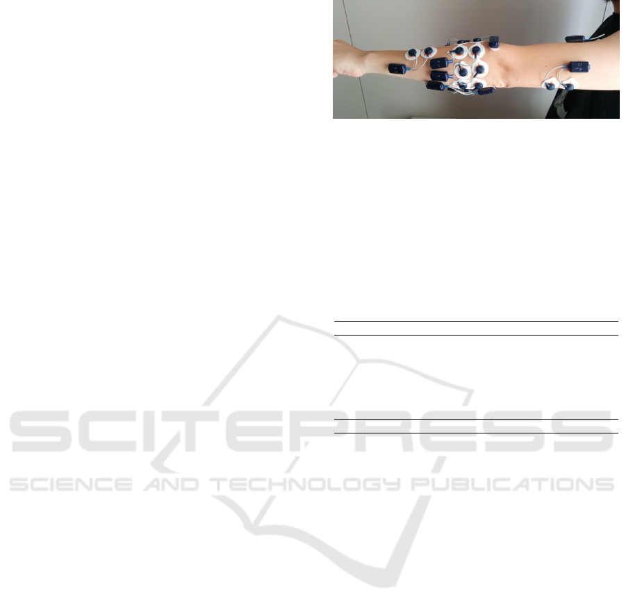
Every sensor is connected to 2 Dormo SX-30 ECG

electrodes with 30mm diameter, covering the forearm

circumference without overlap and assuming the po-

sitions shown in the Figure 1 (Pizzolato et al., 2017;

Atzori, 2014).

The data is divided into 3 classes of movements:

basic wrist movements and isometric hand positions;

grasp and functional movements; and basic ﬁngers

movements. Myoelectric signal is acquired using

12 wireless electrodes: 8 around the forearm in an

equally spaced disposition in correspondence to the

radio humeral joint, 2 electrodes are placed on the

main activity spots of the ﬂexor digitorum and of the

extensor digitorum, 1 on the biceps and 1 on the tri-

ceps (Pizzolato et al., 2017; Atzori, 2014).

Figure 1: Electrode positions, adapted from (Pizzolato

et al., 2017).

Subjects performed 6 repetitions of 52 different

movements using their dominant hand. Each repeti-

tion consisted of 5 seconds of movement and 3 sec-

onds of resting (Pizzolato et al., 2017; Atzori, 2014).

Of the 52 movements, 11 were selected and grouped

into 3 sets, which are described in Table 1 and illus-

trated in Figure 2.

Table 1: Description of the movements included in each set.

Set 1 Set 2

Closed hand (B6) Thumb up (B1)

Wrist supination (B9) Closed hand (B6)

Wrist pronation (B10) Pointing index (B7)

Wrist ﬂexion (B13) Wrist ﬂexion (B13)

Wrist extension (B14) Wrist extension (B14)

Grasp (small diameter) (C2) Ring grasp (C6)

Set 3

Extension of index and middle, ﬂexion of others (B2)

Abduction of all ﬁngers (B5)

Closed hand (B6)

Wrist ﬂexion (B13)

Wrist extension (B14)

Ring grasp (C6)

For our classiﬁcation network, we used as inputs

the EMG data from the main activity spots of the

ﬂexor and extensor digitorum superﬁcialis muscles

of 6 healthy subjects. EMG signals were segmented

based on the repetition variable, which indicates when

the subject is actually performing the gesture and also

give us the repetition number. Since data from the Ni-

napro Project database is provided in .mat ﬁles, we

converted each repetition signal from each movement

to a .csv ﬁle using Matlab, resulting in 3744 .csv ﬁles.

Figure 3 shows an example of one ﬁltered surface

EMG signal that composes the dataset.

Using the data from the dataset 4 of the Ninapro

Database, we created 4 sets: 1 training set and 1 test

set for each of the 2 selected muscles. Since each sub-

ject from the NinaPro database performed 6 repeti-

tions of each hand gesture, we separated 4 repetitions

as the training set (66.7%), and 2 as the testing set

(33.3%). As we have 6 subjects, there are 24 signals

for training and 12 for testing, for each movement.

After performing the aforementioned preprocess-

BIOSIGNALS 2019 - 12th International Conference on Bio-inspired Systems and Signal Processing

186

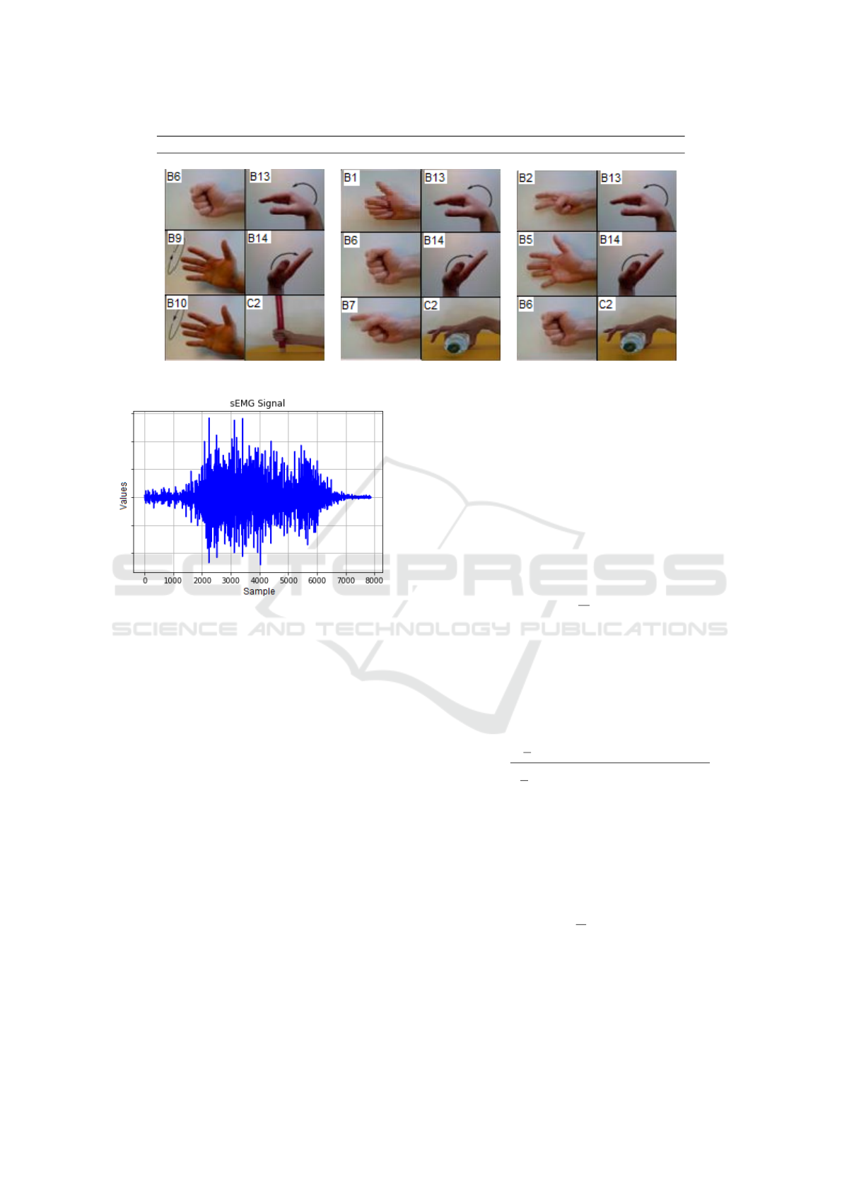
Set 1 Set 2 Set 3

Figure 2: Hand movements performed by subjects.

Figure 3: Example of an surface EMG signal.

ing in Matlab, only Python scripts were used to train

and evaluate the neural network.

2.2 Parameter Extraction and Feature

Scaling

For the EMG signals that composed the dataset, 7 pa-

rameters were calculated to serve as inputs for our

neural network. In the time and frequency domain,

they are the arithmetic mean, the kurtosis, the root

mean square (RMS), the skewness, the standard de-

viation, the variance and the signal energy. In the

frequency domain, there is also the spectral centroid.

These parameters were chosen based on the literature

urigo, 2014; Tang et al., 2012; Nilson, 2014). Af-

ter parameter extraction, the feature scaling method

was used. This is done to even the data to a mean

value of 0 and a standard deviation of 1. This mini-

mizes the potential danger of large numbers (like vari-

ance or the spectral centroid) dominating over small

numbers and to avoid computational difﬁculties dur-

ing calculations (B

urigo, 2014). In the remainder of

this subsection, we present the deﬁnition of each pa-

rameter and the equations used to calculate them. In

the equations shown, f

is the sampling rate, RMS(s)

is the root mean square value of a vector s, N is the

size of the respective array, emg

mean

is the mean value

of the respective array (emg array), and emg(n) is the

element of array emg.

2.2.1 Energy

The energy is calculated by multiplying the squared

RMS value by the time it exists, as shows Equation 1.

Energy =

× RMS(s)

(1)

2.2.2 Kurtosis

The kurtosis is a measure that determines the tailed-

ness of a probability distribution of a random variable.

It is deﬁned as in Equation 2 (B

urigo, 2014).

Kurt[X] =

∑

n=1

(emg(n) −emg

mean

)



∑

n=1

(emg(n) −emg

mean

)



(2)

2.2.3 Mean Value

The mean value is the sum of all elements of an ar-

ray divided by the number of elements, deﬁned as in

Equation 3 (B

urigo, 2014).

emg

mean

∑

n=1

emg(n) (3)

2.2.4 Root Mean Square

The Root Mean Square is also known as the quadratic

mean, simply being the square root of the mean

An Artiﬁcial Neural Network for Hand Movement Classiﬁcation using Surface Electromyography

187

square of a set of data values, calculated as in Equa-

tion 4 (B

urigo, 2014).

RMS =

∑

n=1

emg(n)

(4)

2.2.5 Skewness

Skewness measures the asymmetry of the probability

function of a random variable, which in our case is

our sEMG signal. It is calculated as in Equation 5

urigo, 2014).

Skewness =

∑

n=1

(emg(n) −emg

mean

)



∑

n=1

(emg(n) −emg

mean

)



(5)

2.2.6 Spectral Centroid

The spectral centroid is deﬁned as the center of mass

of the spectrum. Given a array of magnitudes in the

frequency domain, the centroid is calculated as in

Equation 6 (B

urigo, 2014).

Centroid =

∑

n=1

n × emg(n)

∑

n=1

emg(n)

(6)

2.2.7 Standard Deviation

The standard deviation is the measure that quantiﬁes

the variation or dispersion of a set of data values. It is

calculated as in Equation 7 (B

urigo, 2014).

σ =

N − 1

∑

n=1

(emg(n) −emg

mean

)

(7)

2.2.8 Variance

The variance, as the formula suggests, is also a mea-

sure of the dispersion of a dataset similar to the stan-

dard deviation. It is calculated as in Equation 8

urigo, 2014).

N − 1

∑

n=1

(emg(n) −emg

mean

)

(8)

2.3 Neural Network

The brain is a very complex and nonlinear infor-

mation processing system, capable of organizing its

small pieces of structure called neurons to perform

much better than any existing digital computer. This

is possible because the brain is able to connect the

neurons into a huge net called neural network us-

ing electrical signals that travel through a small gap

between the neurons, the synapse. Changing the

synapses will also change the inﬂuence of one neuron

on another and therefore change the brain’s response

to a stimulus (Sousa, 2011) (Haykin, 1999).

In an attempt to biomimic the brain and its struc-

ture the Artiﬁcial Neural Network (ANN) was cre-

ated. This network is an electronic circuit or a soft-

ware that uses massive connection of neurons to per-

form useful computations. The system receives an

input and through its connections and activations an

output is generated. ANNs have the ability to learn

through methods called learning algorithms. It can

also generalize the training, i.e. it can generate a rea-

sonable output with an input that has not been used in

its training (Haykin, 1999).

Figure 4 shows how a ANN is constructed. The

circles represent the neurons, the arrows represent the

synapses, the circle’s superscripts represent its layer

and its subscript represents the neuron number. The

layer 1 represents the input layer, and layer L rep-

resents the output layer. Neurons in the ﬁrst row

(with subscript 0) are the bias neurons, which al-

ways produce the same value and don’t have incom-

ing synapses; the layers that are not input or output

layers are called the hidden layers. N(α) denotes the

number of neurons in the α

layer. The ANN im-

plemented in this work has 1 hidden layer with 12

neurons, with a bias neuron at the input layer and in

the hidden layer. This topology was chosen by tests

measuring the accuracy of 9 different topologies (with

1 and 2 hidden layers) over one of the datasets. It

receives 26 inputs (13 parameters from 2 electrodes)

and outputs 6 numbers, which represent the probabil-

ity of the input being from one of the six movements

in each movement set.

The values in the input layer are forwarded to the

next layer through the synapses. In the ﬁrst layer

(layer 1), the input vector is [a

,. . . ,a

N(1)

]. Each el-

ement of this vector is multiplied by a synaptic weight

, and they are all added to generate the next layers’

neurons’ inputs. The activation function is applied to

this input, creating the neuron output. Each neuron

output value is calculated by Equation 10, with σ as

the sigmoid function (shown in Equation 9), which is

used as the activation function of the neurons. This is

called the feed-forward algorithm.

σ(x) =

1 + e

(x) = σ(x)(1 − σ(x))

(9)

BIOSIGNALS 2019 - 12th International Conference on Bio-inspired Systems and Signal Processing

188

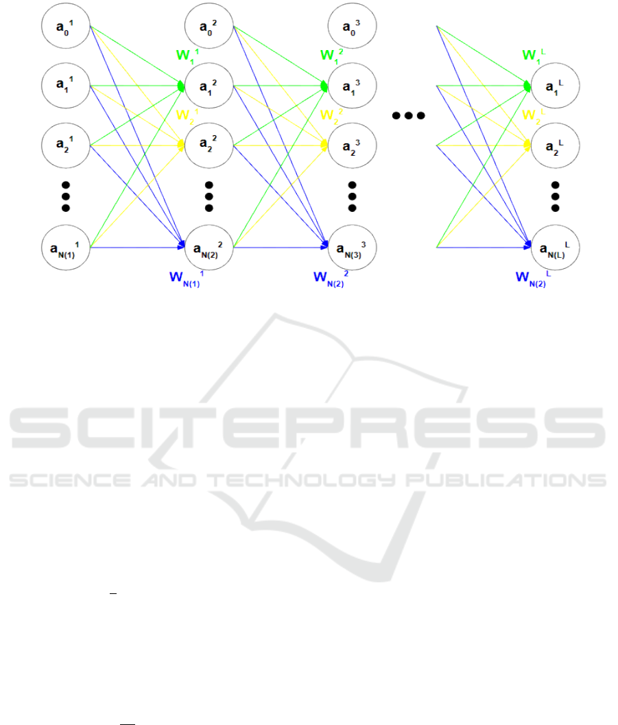
Figure 4: Artiﬁcial Neural Network diagram.

=σ

N( j)

∑

k=0

j−1

∗W

j−1

[k]

i ∈ [0,N( j)]

j ∈ [2, L]

(10)

The training algorithm used in this work is the

backpropagation algorithm. It is considered the algo-

rithm that brought light to neural networks, because

it is a computationally efﬁcient method to train them

(Haykin, 1999). It calculates the partial derivatives

of the error signal with respect to the weights in the

synapses. This value is then summed to the weights

to minimize the error function E(w):

E(w) =

∑

n=1

k y(x

, w) −t

(11)

When we minimize this error, the ANN ap-

proaches its desired behavior. The backpropagation

algorithm work as follows. Given an input x

and

a target output t

, the real output y

of the ANN is

taken using the feed-forward algorithm, as shown in

Equation 10. The derivative of the error in the output

layer is calculated by

∂E

∂a

= t

−y

. From layer L−1 to

layer 1, the partial derivatives are calculated consider-

ing the values of the next layers’ errors and synaptic

weights that goes from the current layer to the next.

The mathematical steps and details are described by

Haykin, 1999.

The training set of the neural network has an in-

put vector x

associated to their corresponding target

vector t

, where n = 1, ...,N and N is the number of

samples in the input. The training stage has the objec-

tive of minimizing the error function in Equation 11

(Bishop, 2006). The hit rate percentage is calculated

by the number of right guesses divided by the total

number of signals to guess.

Having K > 2 separable binary classiﬁcations, it

is possible to apply a neural network with K outputs,

also considering that each output has sigmoid as acti-

vation function and has a binary class label t

∈ [0, 1],

where k = 1, ..., K, associated to it. Due to the input

vector, it can be considered the class labels as inde-

pendent and, therefore, the conditional distribution of

the targets is given by the Equation 12 (Bishop, 2006).

p(t|x, w) =

∏

k=1

(x, w)

[1 − y

(x, w)]

1−t

(12)

Then, the error function with more than one in-

put, originated by applying the negative logarithm in

the likelihood function, results in Equation 13, where

, w) indicates the value in the k-unity in the n-

example, and t

is the expected value in the k-unity

in the n-example (Bishop, 2006).

E(w) = −

∑

n=1

∑

k=1

∗ ln(y

, w))+

(1 −t

) ∗ ln(1 −y

, w))

(13)

In neural networks literature, there is the conven-

tion of considering the minimization of the error func-

tion instead of the maximization of the likelihood, but

both methods are equivalent (Bishop, 2006).

An Artiﬁcial Neural Network for Hand Movement Classiﬁcation using Surface Electromyography

189

An Artiﬁcial Neural Network class was created in

Python programming language, using few and sim-

ple libraries. This is good for portability, in such a

way that a embedded system, for instance, would not

need to have installed a number of big libraries just for

using one feature of it, reducing hardware complex-

ity. The number of epochs during the training phase

was chosen empirically, in such a way that the ANN

reaches about 99% hit rate at the training set (after

this, the ANN will start overﬁtting). All codes related

to the artiﬁcial neural network creation, training and

evaluation were coded in Python language. The mod-

ules used are listed below:

• numpy

• numpy.fft

• csv

• scipy.signal

• scipy.stats

• cProﬁle

• matplotlib.pyplot

• random

• time

The codes were written in Python 2.7, and Spy-

der IDE version 3.2.6 was used to write, test and run

them. Spyder is ”a powerful scientiﬁc environment

written in Python, for Python, and designed by and for

scientists, engineers and data analysts” (as described

in Spyder Website). Spyder was used within Ana-

conda, a platform for Python and R data science and

machine learning, according to the Anaconda web-

site. All of this was processed on a Windows 10,

64bits machine, i5-4210U 2.4GHz CPU.

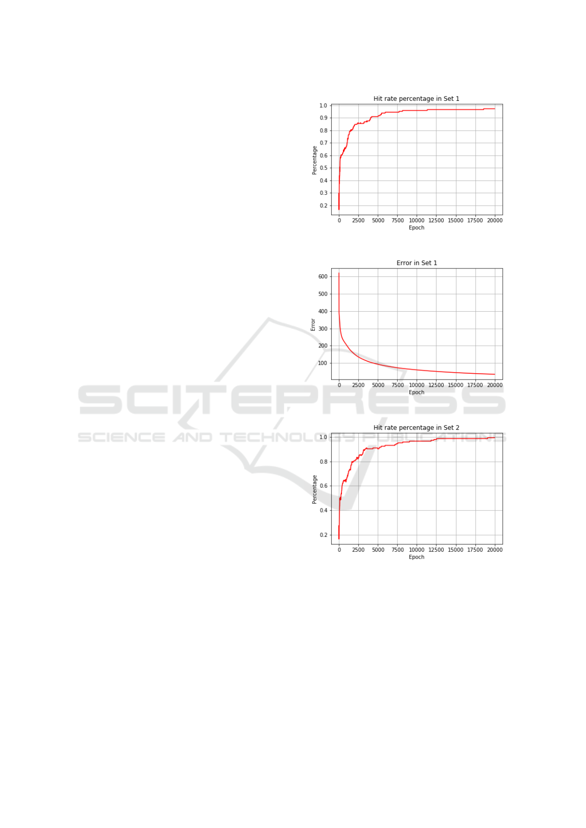
3 RESULTS

Figure 5 shows the hit rate by training epoch, while

Figure 6 shows the error by training epoch for move-

ment set 1. As we can see, the hit rate reaches 100%,

while the error decreases below 30. This number is

less important than the actual hit rate, but has interest-

ing implications, as we will see in Section 4. For this

dataset, the testing set hit rate achieved was 86.11%.

Figures 7 and 8 show the hit rate and error by

epoch for the training phase for movement set 2. The

hit rate in the testing set was 88.89%.

Figures 9 and 10 show the hit rate and error by

epoch for the training phase for movement set 3. The

hit rate achieved with this set was 87.5%.

The hit rate is a natural measure of the classiﬁ-

cation method, but it does not account for mistakes

Figure 5: Hit rate achieved using set 1.

Figure 6: Error during training in set 1.

Figure 7: Hit rate achieved using set 2.

made by samples of a class over another class (Nil-

son, 2014). To verify which movements the ANN

classiﬁed correctly and which ones it did not, we con-

structed a confusion matrix for the movement set 1.

In this matrix, the columns show the actual move-

ment and the row shows which movement the ANN

guessed. As we can see in table 2, the ANN did

not have much problem classifying movements B6,

B13, B14 and C2, and had a lower hit rate classi-

fying movements B9 and B10. As we can see, the

ANN mistook movements B10 for B9 and B9 for B10

BIOSIGNALS 2019 - 12th International Conference on Bio-inspired Systems and Signal Processing

190

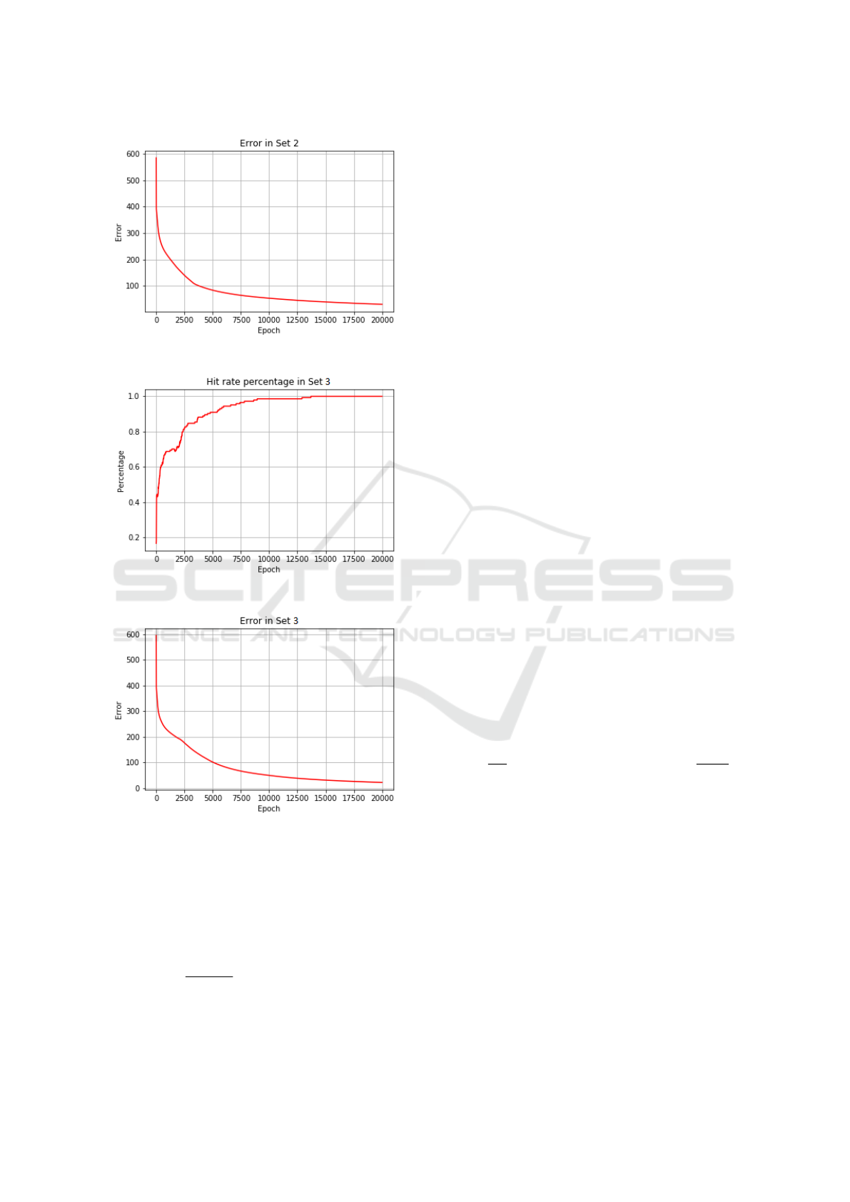
Figure 8: Error during training in set 2.

Figure 9: Hit rate achieved using set 3.

Figure 10: Error during training in set 3.

more often (wrist supination and pronation), which is

understandable because they are very similar move-

ments. Wrist supination had the lowest hit rate.

The classiﬁcation time of the ANN was also mea-

sured. For this, the feed-forward algorithm was ap-

plied to the training set (144 repetitions) 10000 times.

The time measured was 173.596 seconds, what makes

an average of

16.55s

144∗10000

= 120.6µs spent on each repe-

tition. The time of reading the data from the .csv ﬁles,

pre-processing them, separating the movements of the

training and testing sets, and extracting the parame-

Table 2: Confusion Matrix for movement set 1.

Actual movement

B6 B9 B10 B13 B14 C2

Guessed mov.

B6 10 0 0 1 0 0

B9 0 7 2 0 0 0

B10 0 2 8 0 1 0

B13 0 1 1 10 0 0

B14 0 1 0 0 11 0

C2 2 1 1 1 0 12

ters was also measured as 200.19 seconds. The train-

ing time (during 20000 epochs) was 1064.97 seconds,

making an average of 53.2ms per epoch or 18.78

epochs per second. It’s important to note that our code

reads all the 52 movements from the dataset and only

saves in variables the movements that will be used to

train the ANN.

4 DISCUSSION

The hit rate for movement set 3 (the same as (Tang

et al., 2012)) was 87.5%. This means an 9.6% hit

rate increase compared to (B

urigo, 2014), and a de-

crease of 7.3% compared to (Tang et al., 2012), us-

ing a smaller number of electrodes. This reduction in

the number of electrodes brings many advantages to

a potential application in a myoelectric controlled de-

vice. It translates into less discomfort for the user, less

computational processing needed, less battery usage,

lower costs and weight.

We can notice that the error (from Equation 13)

achieved in sets 1, 2 and 3 was below 30. We can il-

lustrate the signiﬁcance of this with an example. With

an error of 30, with 144 repetitions (6 subjects with 6

movements and 4 repetitions for each movement, in

the training set), the mean contribution of each move-

ment is

−30

144

= −0.208, and of each guess is

−0.208

−0.0347. Taking the exponential of this number (cal-

culating equation 13 backwards) and knowing that the

ANN output can be interpreted as the probability of

the guess being the right guess, we can see that the av-

erage “conﬁdence” of the ANN is e

−0.0347

= 96.6%.

For instance, if this average was 60%, this error would

be −308.2.

We proposed using a feed-forward Neural Net-

work to solve the problem boarded in this work. How-

ever, there are many types of Neural Networks used

for Supervised Learning in the literature, such as

Convolutional Neural Networks and Recurrent Neu-

ral Networks. The former is used for the recognition

of 2D shapes (Haykin, 1999), which is not the case,

while the second could indeed be used for this kind of

task. However RNNs need many layers and more data

An Artiﬁcial Neural Network for Hand Movement Classiﬁcation using Surface Electromyography

191

preprocessing, what would increase the training time.

Using time windows of 200 samples and assuming

just 1 second of gesture duration, with a sampling rate

of 2kHz, each gesture repetition would generate 1800

sets of 200 features per electrode (1800 sequences of

200 sampled signals), instead of our 1 set of 13 fea-

tures per electrode. This approach can be investigated

in a future work.

During coding and testing, the Python module

cProﬁle was used to identify which functions were

spending more time in the processor unit, enabling us

to ﬁne tune some functions and methods to increase

overall performance. Additionally, using the sigmoid

as activation function had the beneﬁt of reducing the

time spent on training the network, because its deriva-

tive can be written as a function of the function itself,

whose value was already calculated and stored.

Our neural network classiﬁer proved to be very

fast, classifying sample signals in less than 1 ms.

It also does not need a lot of computational mem-

ory, because it only needs to store the weights in the

synapses after the training is complete. Reduced run-

time and complexity are valuable features, as they

help ensure the system has a reasonable response

time. Ideally, the delay introduced by a control sys-

tem should not be perceived, being kept below a

threshold of roughly 300 ms. However, there is a

trade-off between run-time, complexity and accuracy,

with the latter being critical for a correct operation.

This compromise should be considered in the design

of any system controlled by myoelectric signals (En-

glehart and Hudgins, 2003).

5 CONCLUSION

In this paper, we presented the development of a rela-

tively simple ANN that can classify hand movements

and gestures using surface EMG data from a reduced

number of electrodes. We achieved a hit rate of above

80% in all 3 test sets, with a maximum of 88.89% for

movement set 2, with small system complexity and

run time.

Future works may investigate how additions to

this ANN, such a regularization method, can be im-

plemented to improve its performance. The efﬁ-

cacy of the proposed ANN’s performance on a big-

ger dataset with more subjects and a greater num-

ber of movements may also be examined in order

to test the ANN’s generalization power. Another in-

teresting possibility is to compare the performance

of the proposed ANN with different machine learn-

ing algorithms of similar complexity, number of in-

puts and computational time using the same dataset.

This could potentially generate a group of simple, fast

classiﬁers that combined, may achieve higher perfor-

mance levels.

REFERENCES

Atzori, M. (2014). Ninapro website. http://ninapro.hevs.ch/.

[Online]; accessed on October 21, 2018.

Bishop, C. (2006). Pattern Recognition and Machine

Learning, volume 29.

urigo, A. (2014). Classiﬁcac

ao de Movimentos de M

Utilizando Eletromiograﬁa de Superf

ıcie, Regress

Log

ıstica, Redes Neurais, M

aquina de Vetores de Su-

porte e Base de Dados NinaPro.

Englehart, K. and Hudgins, B. (2003). A Robust, Real-Time

Control Scheme for Multifunction Myoelectric Con-

trol. IEEE Transactions on Biomedical Engineering,

50(7):848–854.

Guyton, A; Hall, J. (2010). Textbook of Medical Physiology.

Haykin, S. (1999). Neural Networks: A Comprehensive

Foundation. Prentice Hall.

Nilson, C. D. E. P. (2014). Aquisic¸

ao, Processamento de

Sinais Mioel

etricos e M

aquinas de Vetores de Su-

porte para Caracterizac¸

ao de Movimentos do Seg-

mento M

ao-Brac¸o.

Pizzolato, S., Tagliapietra, L., Cognolato, M., Reggiani, M.,

Mller, H., and Atzori, M. (2017). Comparison of six

electromyography acquisition setups on hand move-

ment classiﬁcation tasks. PLOS ONE, 12(10):1–17.

Sousa, D. (2011). How the Brain Learns. SAGE Publica-

tions.

Tang, X., Liu, Y., Lv, C., and Sun, D. (2012). Hand mo-

tion classiﬁcation using a multi-channel surface elec-

tromyography sensor. Sensors, 12(2):1130–1147.

BIOSIGNALS 2019 - 12th International Conference on Bio-inspired Systems and Signal Processing

192