Predicting the Early Stages of the Alzheimer’s Disease via Combined

Brain Multi-projections and Small Datasets

Kau

e T. N. Duarte, Pedro V. V. de Paiva, Paulo S. Martins and Marco A. G. Carvalho

School of Technology, University of Campinas (UNICAMP), R. Paschoal Marmo, Limeira, Brazil

Keywords:

Classiﬁcation, Transfer Learning, Mild Cognitive Impairment, Clinical Dementia Rating, Support Vector

Machines.

Abstract:

Alzheimer is a neurodegenerative disease that usually affects the elderly. It compromises a patient’s memory,

his/her cognition, and perception of the environment. Alzheimer’s Disease detection in its initial stage, known

as Mild Cognitive Impairment, attracts special efforts from experts due to the possibility of using drugs to

delay the progression of the disease. This paper aims to provide a method for the detection of this impairment

condition via the classiﬁcation of brain images using Transfer Learning - Deep Features and Support Vector

Machine. The small number of images used in this work justiﬁes the application of Transfer Learning, which

employs weights from VGG19 initial layers used for ImageNet classiﬁcation as deep features extractor, and

then applies Support Vector Machines. Majority Voting, False-Positive Priori, and Super Learner were applied

to combine previous classiﬁers predictions. The ﬁnal step was a detection to assign a label to the previous

voting outcomes, determining the presence or absence of an Alzheimers pre-condition. The OASIS-1 database

was used with a total of 196 images (axial, coronal, and sagittal). Our method showed a promising performance

in terms of accuracy, recall and speciﬁcity.

1 INTRODUCTION

The Alzheimer’s Disease (AD) is a neurodegenera-

tive dementia that affects the human abilities related

to memory, language, perception of the environment

and cognitive skills(Ferreira and Busatto, 2011). Mild

Cognitive Impairment (MCI) is known as a prodromal

stage of AD and corresponds to the range between a

normal aging and dementia. MCI is gaining atten-

tion because by predicting the disease in this stage,

patients are able to ﬁnd out ways to slow down the di-

sease. Besides, this stage is relevant due to its strong

relationship with the AD progression. As a matter of

fact, 10-12% of the MCI cases convert to AD each

year (Petersen et al., 1999).

The most popular term used to classify speciﬁc

stages in the MCI is the Clinical Dementia Rating

(CDR), deﬁned by the following levels: CDR-0 repre-

sents Normal Control (NC) or non-dementia people;

CDR-0.5 corresponds to a very mild dementia; CDR-

1 represents a mild impairment dementia; CDR-2 is

a moderate dementia, whereas CDR-3 indicates se-

vere dementia. These levels allow the medical team to

identify a better prognostic for the AD patient. They

also facilitate the process of classifying images.

Different analysis are currently used to diagnose

or predict AD, such as: (1) Family History; (2) Ima-

ging; (3) Cognitive Tests (Mini-Mental State Exami-

nation); and (4) Neurological Exams.

This work uses imaging to support the prediction

of the Alzheimers disease through the detection of

MCI, which is one indicator of early signs of AD. It is

very difﬁcult to predict AD using only one projection

of the brain (e.g. sagittal). Thus, the combination of

the different planes of the brain, also known as multi-

projection, is used and has reached higher accuracy

than single-projection frameworks (Aderghal et al.,

2017)(Zhou et al., 2017). The results in the litera-

ture achieve higher accuracy also when comparing

some stages of the disease, for instance, when com-

paring CDR-0 and CDR-3 patients (Khedher et al.,

2015)(Suk and Shen, 2016). However, our work fo-

cus on the two initial stages (i.e. CDR-0.5 and CDR-

1) due to our emphasis on predicting the AD dementia

as soon as possible. An example of brain atrophy is

shown in Figure 1.

In this work, we aim at classifying MCI images

using visual information and a small number of sam-

ples. Image data was analyzed using Transfer Lear-

ning with Convolutional Neural Networks (CNN) and

Duarte, K., V. de Paiva, P., Martins, P. and Carvalho, M.

Predicting the Early Stages of the Alzheimer’s Disease via Combined Brain Multi-projections and Small Datasets.

DOI: 10.5220/0007404705530560

In Proceedings of the 14th International Joint Conference on Computer Vision, Imaging and Computer Graphics Theory and Applications (VISIGRAPP 2019), pages 553-560

ISBN: 978-989-758-354-4

553

(a) (b)

Figure 1: Brain Status (on Aging, 2016): (a) healthy subject

(CDR-0), (b) subject with severe Alzheimer (CDR-3).

Support Vector Machine (SVM).

The main features and contributions of this work

are: (1) The combination of Transfer Learning, SVM,

and Voting for small datasets; (2) The Grouping of

MCI classes to improve the number of images per

class (i.e. thus facilitating the identiﬁcation of pat-

terns); (3) Application of our approach to the ﬁrst sta-

ges of MCI, which turns the discrimination of AD a

more challenging task; (4) The availability of the code

and the implementation used to generate this paper.

The remainder of this paper is organized as fol-

lows: In Section 2 we address related work. The pro-

posed method, the fundamentals and details of each

step in the method are addressed in Section 3. The ex-

periments and the evaluation of the method are shown

in Section 4. Finally, in Section 5 we present our con-

clusions.

2 RELATED WORK

Different computational methods using textual data

or visual information have been applied in the me-

dical ﬁeld. For example, Lebedev (Lebedev et al.,

2014) address the problem of diagnosing AD using

Random Forest (RF) classiﬁers and different measu-

res obtained from clinical Magnetic Resonance Ima-

ging (MRI) data. The best performance was achieved

with RF and it reached an accuracy over 90% by com-

paring AD with NC images.

The use of a CNN is presented by Wang (Wang

et al., 2017) to automatically recognize MCI in MRI.

The authors addressed the problem of limited training

data using data augmentation and transfer learning to

pre-train the proposed CNN model. Three different

datasets were used for the training and classiﬁcation

stages: OASIS, LIDC, and ADNI, The authors repor-

ted an accuracy of 90,6% and a F-score of 89,4%.

There is a body of work that combines information

from different modalities or projections. When dea-

ling with the prediction of the AD (Normal, MCI and

AD levels), Fiot (Fiot et al., 2012) employs the use

of Laplacian EigenMaps in order to reduce the data

dimensionality and the K-Nearest Neighbor (KNN)

classiﬁer. They used the MRI, one protein, and six ge-

notype data from the ADNI dataset and reached accu-

racies from 62% up to 83% when comparing Normal

and MCI classes.

Khedher (Khedher et al., 2015) used the data pro-

vided by ADNI dataset to compose a multivariate

method with Partial Least Squares, Principal Compo-

nent Analysis and SVM. Aderghal (Aderghal et al.,

2017) proposed a multi-projection fusion of Axial,

Coronal and Sagittal CNNs using Regions of Interest.

The accuracy reached was 85,94% when comparing

AD and NC. In Suk and Shen (Suk and Shen, 2016),

the authors proposed a framework based on sparse re-

gression as learner representation. Thus, they built a

CNN for clinical decisions. An accuracy of 90,28%

was reached by their method. Using Positron Emis-

sion Tomography (PET) images instead of MRI scans,

Gray (Gray et al., 2011) proposed a region-based ana-

lysis of AD patients, using segmentation of 83 ana-

tomical regions obtained by MRI. The authors used

SVM to classify samples and reached an accuracy of

82% when comparing AD and NC. Cheng and Liu

(Cheng and Liu, 2017) proposed a method based on

2D-CNN to learn features from 3D PET images, and

they achieved an accuracy of 91,40 % .

Some of the literature reviewed in this section rea-

ched a relative high accuracy since they compare NC

and AD images. Clearly, AD images possess more

discriminative features of the disease than MCI ima-

ges. For example, in Khedher (Khedher et al., 2015),

the results obtained by the comparison of NC and

MCI reached an accuracy of 80,27%. On the other

hand, when comparing only the NC and AD classes,

the accuracy was increased to 88,49%. Our work deﬁ-

nes a scenario with a focus on MCI, which represents

the initial levels of disease.

In essence, our work differs from previous works

by the following features: (1) the use of Transfer Le-

arning (TL) instead of fully-CNNs. The TL-CNNs

have not been previously applied within the same con-

text of this work; (2) the use of the ﬁrst two classes

of MCI (i.e. CDR-0.5 and CDR-1). The most chal-

lenging prediction of the early stages of the Alzhei-

mer disease via classiﬁcation lies within the ﬁrst clas-

ses because these images are quite similar to those

from healthy individuals; (3) the proposed method re-

ached satisfactory results even when using a small set

of images.

VISAPP 2019 - 14th International Conference on Computer Vision Theory and Applications

554

3 PROPOSED METHOD

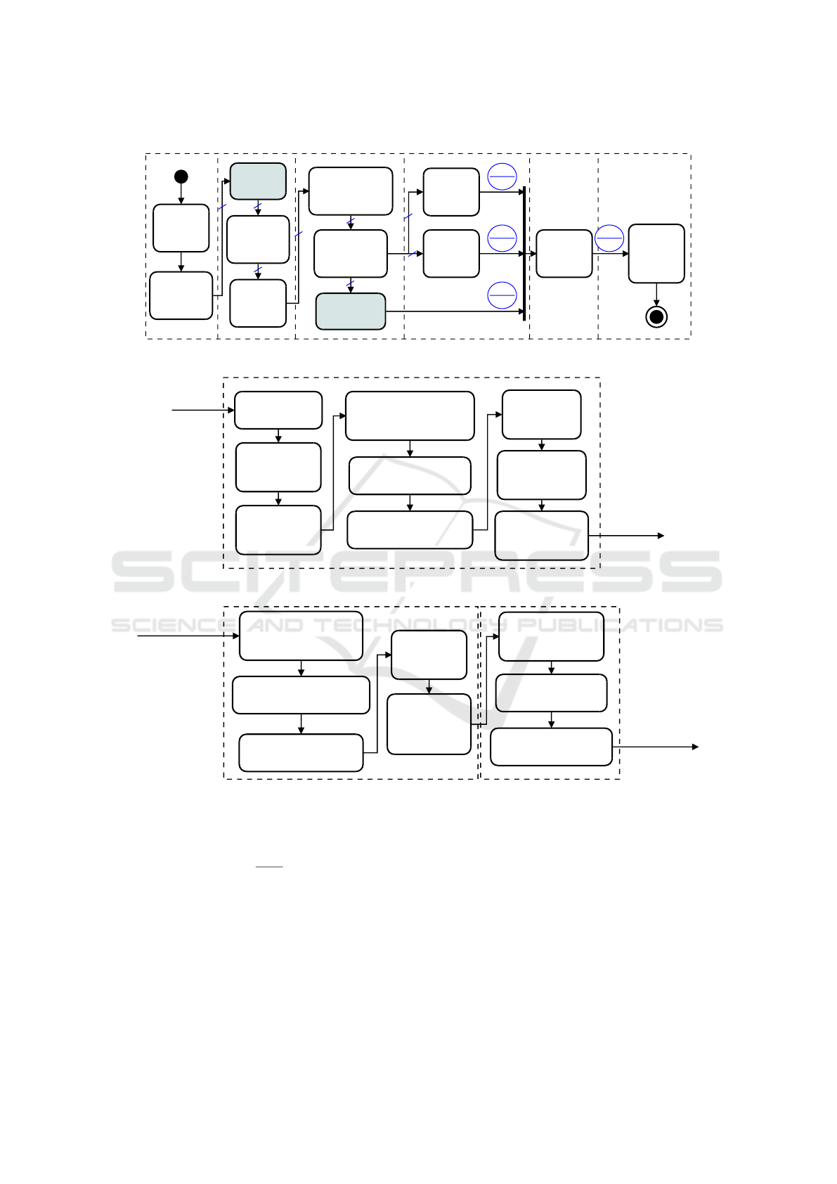
We arranged the method in six major steps (Figure

2): (1) Input data: including acquisition and cate-

gorization; (2) Preprocessing: it involves skull strip-

ping, image enhancement, and data normalization;

(3) Classiﬁcation: it combines Transfer Learning and

SVM. Super Learner was also applied to the SVM

outputs; (4) Voting: the method applied Majority Vo-

ting and False-Positive Priori to the outputs of SVM;

(5) Detection: it also applies Majority Voting to the

inputs and it labels the samples combining the previ-

ous procedures; (6) Output: generate a label deﬁning

either the presence or the absence of MCI.

Our method (Figure 2(a)) starts out by extracting

each slice of a 3D-brain projection. The MCI classes

are grouped using Spectral Clustering (Figure 2(b)).

Thus, the skull is removed and the intensity adjus-

ted. For the sake of classiﬁcation, Transfer Learning

is applied in each representation to generate deep fea-

tures, which are further used in SVMs to classify ima-

ges. Methods such as Majority Voting, FP Priori, and

Super Learner are used to combine the results of the

projections. Finally, Majority Voting is carried out to

group the results of each method. The ﬁnal response

is the detection whether a subject has MCI or not.

In Figure 2(a), each crossed blue line with identi-

ﬁer three (3) informs the number of projections in the

ﬂow. Also, in each blue circle, the upper part means

an example of response for each projection (i.e. axial,

coronal, and sagittal), whereas the lower part shows

the result after voting or classiﬁcation. We now dis-

cuss each step of the method in more detail.

3.1 Input Data

In this work, the Open Access Series of Imaging Stu-

dies (OASIS)-1: Cross-sectional MRI Data in Young,

Middle Aged, Nondemented and Demented Older

Adults was used. The CSV ﬁle dataset is formed by

436 subjects data (135 NC, 70 CDR-0.5, 28 CDR-

1, 2 CDR-2, and 201 unlabeled) with age between

18 and 96 years. For each patient, the following in-

formation is given: (1) Demographic: Age, gender,

education, Socioeconomic Status (SES); (2) Clini-

cal: Mini-Mental State Examination (MMSE), Cli-

nical Dementia Rating; (3) Derivated anatomic vo-

lumes: estimated Total Intracranical Volume (eTIV),

Atlas Scaling Factor (ASF), normalized Whole Brain

Volume (nWBV); and (4) Imaging: Magnetic Reso-

nance Imaging. The above related text data were or-

ganized in a table in order to facilitate the data mining

interpretation.

Each subject is associated with a 208x176x176

pixel image. Three slices from different views of the

brain were extracted: (1) The Axial MRI, which is

composed of 208 x 176 pixels (slice #90); (2) Coro-

nal MRI, consisting of 176x176 pixels (slice #110),

and (3) Sagittal MRI with 208x176 pixels (slice #95).

The extraction of each brain projection is showed

in the Figure 3.

3.2 Preprocessing

Preprocessing plays a key role in every classiﬁer’s

performance. In this work, the same preprocessing

ﬂow was applied to each individual brain projection,

which were programmatically extracted from the ori-

ginal 3D brain representation.

3.2.1 Grouping of the MCI Classes

This step employed information provided by the OA-

SIS dataset, which consists of clinical, demographic,

and functional information of subjects. The algorithm

used for grouping the MCI-classes (in step 5) was

Spectral clustering. It required four preparation steps,

i.e. steps 1-4 for data cleaning and transformation:

1. Removal by age: Guerreiro (Guerreiro and Bras,

2015) indicated that the brain has a normal

atrophy due to aging. Thus, a healthy 96 year-old

brain shows discriminative values in relation to an

18-year-old brain. The authors also point out that

AD commonly occurs at age 65 or older. In order

to avoid misclassiﬁcation, 238 subjects under age

60 were removed from the original dataset with

436, thus remaining 198 subjects.

2. Removal by classes: Two subjects classiﬁed as

CDR-2 were also removed, thus remaining 196

subjects. The goal was to avoid mislabeling due

to the small number of samples;

3. Data ﬁlling: 19 subjects had no SES informa-

tion. Instead of removing these data, this condi-

tion was mitigated by adding values using Pro-

gressive Sampling and Linear Regression;

4. Data transformation: The goal is to ﬁt the data

for the Spectral Clustering inputs using the follo-

wing steps: (a) Scale adjustment: The eTIV and

nWBV attributes were originally speciﬁed in dif-

ferent scales. Thus, if the data were below a cer-

tain threshold (10 in our case), they were multip-

lied by 10

; (b) Attribute binarization: The Gen-

der attribute originally had (M/F) categorical va-

lues. They were binarized by setting one (1) for

M and zero (0) for F; (c) Normalization: In order

to assign the same weight to each type of attri-

bute, the data were normalized using the Standard

Score (z-score) (Equation (1)):

Predicting the Early Stages of the Alzheimer’s Disease via Combined Brain Multi-projections and Small Datasets

555

Acquire

3D Brain

Image

Extract 2D

slice of each

projection

Group AD

classes

Extract non-

cerebral

tissue

Enhance

the image

intensity

Generate deep

features using

Transfer Learning

Apply

Support Vector

Machine

Apply

the

FP Priori

Apply the

Majority

Voting

Apply the

Super Learner

1. Input 2. Preprocessing 3. Classification 4. Voting 6. Output

Generate

a Label

(has or

not MCI)

5. Detection

Arbitration

(Decision

Making)

1,0,0

1,1,0

(a)

Group AD classes

Acquire datasheet

in OASIS-1

Remove patients

in 18-59 years

old range

Remove patients

classified as

CDR-2

Update SES information

using Progressive Sampling-

Linear Regression

Normalize eTIV and nWBV

to a same scale

Convert gender from

categorical to binary values

Normalize the

datasheet using

Standard Score

Apply Spectral

Clustering to

find binary classes

Update the classes

according to

above results

from input

block

to Extract

non-cerebral

tissue

(b)

Apply the Super Learner

Split dataset into Training

and Test set using

10-fold cross validation (1)

Divide each training fold using

10-fold cross validation (2)

Generate a classifier using

the new training set (2)

Apply the new

classifier

in Test set (2)

Concatenate the

results of each

classifier into

a vector

using each projection separately

Concatenate all the

classifiers responses

(vectors) into a matrix

Generate a model using

RF in the responses

After applying TL, perform

Super Learner in

using all projections together

from Apply Support

Vector Machine

to Arbitration

(Decision Making)

(c)

Figure 2: Overview of the proposed method for MCI recognition. (a) Entire model for recognition; (b) Grouping of AD

Classes step; (c) Super Learner approach.

~z =

~x − ¯x

, (1)

where ~x represents the data points, ¯x is the mean

value of an attribute, and σ is the standard devia-

tion.

5. Spectral Clustering: The two initial CDR-classes

with dementia (i.e. CDR-0.5 and CDR-1) were

grouped using spectral clustering to create the

group of non-healthy subjects. This technique is

based on a similarity matrix and eigenvalues and

the goal is to perform a reduction in the dimen-

sionality of the data. The outcome is the assign-

ment of the CDR-0 class to one group and both

the CDR-0.5 and CDR-1 classes to another.

3.2.2 Skull Stripping

Also known as Brain Extraction, this step deals with

the removal of non-cerebral tissue from an MRI scan.

The OASIS-1 dataset provides brain images that are

VISAPP 2019 - 14th International Conference on Computer Vision Theory and Applications

556

(a) (b) (c) (d)

Figure 3: 3D representation of the Brain using OASIS-1: (a) Head illustration (adapted from (Lordkaniche, 2011)), (b) Axial

Plane, (c) Coronal Plane, (d) Sagittal Plane.

already extracted. However, brain extraction may be

independently accomplished my means of the Brain

Extraction Tool (Jenkinson et al., 2005).

3.2.3 Intensity Enhancement

The pixels in magnetic-resonance images have dis-

tinct intensities, which requires that the contrast must

be adjusted so that they all fall within the same inter-

val. Thus, the pixels were normalized using a 256-bin

MinMax through Equation (2):

= low

+ (high

− low

) ×

I − low

high

− low

(2)

where I

is the enhanced image, I represents the

original image, high represents the highest-intensity

pixel value, low is the lowest-intensity pixel value, i

and o are reference indexes to input and output data

respectively.

3.3 Classiﬁcation

Classiﬁcation is the problem of identifying to which

of a set of categories (sub-populations) a new obser-

vation (data) belongs. It adds a label to a data sample,

thus assigning it to a speciﬁc set. In this work, the la-

bels are binary as they specify either the presence or

the absence of MCI (i.e. CDR-0.5 and CDR-1).

The two types of classiﬁers used were Transfer

Learning and SVM. SVM’s are used to divide a da-

taset with binary classes in a hyperplane representa-

tion. In this work, we set the SVM using the follo-

wing attributes: C=1.0, kernel = radial basis function.

Since SVM’s are quite well documented in the li-

terature(Hearst et al., 1998)(Cristianini and Shawe-

Taylor, 2000), in this section we focus on Transfer

Learning.

CNN is a speciﬁc type of neural network that uses

grid-topologies as input data, such as images. Un-

like Artiﬁcial Neural Networks, CNNs have Convo-

lutional Layers for the processing of linear functions

and Pooling Layers for the non-linear ones. However,

CNNs have some restrictions: (1) They can only be

performed with a large number of images (i.e. thou-

sands). Depending on the model, the number of weig-

hts can reach millions for each convolutional layer

and their processing demands a relatively high com-

putational effort; (2) In the medical ﬁeld there are few

domains that have large (i.e. enough) amount of avai-

lable data.

TL-CNN is a methodology that transfers pre-

trained network information to another network,

whether it belongs to the same domain or not. It is

an alternative to the application of CNNs when the

datasets are relatively small.

In this work, we used TL-CNN as follows: (1) A

VGG19 pre-trained network using the ImageNet da-

taset was loaded; (2) As the images inside ImageNet

have no relation to our images, only the six ﬁrst layers

were maintained (the ﬁrst layers only extract generic

features); (3) All the layers from the seventh up to the

last one were excluded; (4) Once the images are input

to the neural network, the outputs of the sixth layer

are L matrices with M × N dimension, where L repre-

sents the number of kernels and M × N represents the

image size; (5) Finally, we reshaped the output to one

row per image (also known as deep features).

3.4 Voting

Each method is pooled before a ﬁnal classiﬁcation de-

cision is carried out. In this work, two voting appro-

aches were used: (1) FP Priori: The decision of the

ensemble is TRUE if at least one of the classiﬁers re-

sults in a false-positive (FP). (2) Majority Voting: In-

dividual classiﬁers are combined by taking a simple

majority vote of their decisions. For any given in-

stance, the class chosen by most number of classiﬁers

is the ensemble decision.

Predicting the Early Stages of the Alzheimer’s Disease via Combined Brain Multi-projections and Small Datasets

557

3.5 Detection and Output

The procedure for detection is quite simple: the out-

put of the Majority Voting, the Super Learner and the

FP Priory are submitted to another Majority Voting to

generate the ﬁnal label. The ﬁnal output is a boolean

ﬂag (or label) indicating whether a subject has MCI

(labeled as 1) or not (labeled as 0).

3.6 Software Implementation

The following tools were used for the implemen-

tation of the method: (1) In the Input step, the

208x176x176-pixel images were sliced using the

MATLAB’s r2015b Image Processing toolbox; (2)

The grouping of MCI classes was implemented early

in the preprocessing step using Python 3.4 Jupyter

Notebook, with the Scikit-learn package. Some steps

were manually coded (e.g. Progressive Sampling).

The image enhancement and skull stripping were ge-

nerated using MATLAB; (3) The Classiﬁcation step

was all implemented using Python 3.4 Jupyter Note-

book. The extraction of deep features were obtained

using the Keras toolbox (with TensorFlow backend).

Once the CNN features were extracted, the SVM was

applied using the Scikit-learn package. The Super Le-

arner was manually implemented; (4) In the Voting

step, both the techniques (FP Priori and Majority Vo-

ting) were manually implemented using Python 3.4

Jupyter Notebook. (5) Detection was implemented

using Python 3.4 Jupyter Notebook; (6) Finally, the

metrics were generated using Python 3.4 Jupyter No-

tebook with Scikit-learn package.

All images and codes implemented in this work

are available in the GitHub platform(Duarte and

Paiva, 2018).

4 EXPERIMENTS AND RESULTS

Five metrics were adopted in this work: (1) Precision

- P; (2) Recall - R; (3) F-score - F; (4) Accuracy -

A; (5) Speciﬁcity - S. They are obtained by combi-

ning the true-positive (TP), true-negative (TN), false-

positive (FP), and false-negative (FN) values. These

evaluation metrics are obtained as follows:

P =

T P

T P + FP

, R =

T P

T P + FN

, F = 2 ×

P ∗ R

P + R

(3)

A =

T P + T N

T P + T N + FP + FN

, S =

T N

FP + T N

(4)

The data were ﬁrst divided into a training and test

set by applying a 10-fold cross-validation. After the

results have been obtained, it is performed the average

between metrics using all folds. Thus, reducing the

signiﬁcance of random factors. Regarding the TL-

CNN methodology, the training set was also divided

in 10% for validation and 90% remaining kept trai-

ning set.

To obtain a reasonable accuracy in the voting step,

it is signiﬁcant to ensure that there is a small correla-

tion among the classiﬁer outputs. The correlation ma-

trix for these outputs is illustrated in Table 1. The ana-

lysis using the Pearson Correlation coefﬁcient shows

that the only correlations that are “moderate” are the

Axial and the Coronal (0.72). The correlation bet-

ween the other attributes is considered “weak”. Even

though the correlation between Axial and Coronal is

moderate, we opted to keep the three projections since

it is not possible carry out any decision with only two

projections, i.e. a third projection is always needed

for tie-breaking.

Table 1: Correlation Matrix from classiﬁers’ predictions.

Axial Coronal Sagittal

Axial 1 0.72 0.42

Coronal 0.72 1 0.27

Sagittal 0.42 0.27 1

Table 2 presents the results of our method and

the literature (NC vs MCI) regarding the ﬁve metrics.

When comparing with classiﬁers from literature, the

best ensemble evaluated regarding the speciﬁcity va-

lue was FP Priori (0.754).

The dataset was reduced to prevent any bias in the

classiﬁcation step. For example, the subjects under

60 years were all removed due to their high discrimi-

native patterns in regard to subjects above 60 years.

The CDR-2 samples were also removed due to their

insufﬁcient number (i.e. two), which would cause a

mislabeling at the time the CNN was trained. In the

end, 53% of the samples were removed.

The results are shown in Figure 4. Our method

ranked 5th (FP Priori) for Recall; 4th (Arbitrary) for

Accuracy, and 3rd (FP Priori) for Speciﬁcity. Nevert-

heless, our best result was achieved with the Arbitrary

voting (precision = 0.72, F-Score = 0.716, and accu-

racy = 0.726). It is important to notice that the num-

ber of samples in our case was lower than the others

in the literature (196 x 287 Kheder). Unlike Khed-

her who used ADNI, we used the OASIS dataset. We

have also not extended the data. Among the work re-

viewed in this section, the only that employed multi-

modality was Khedher (Khedher et al., 2015), which

from the literature was the best work evaluated. Ho-

wever, the authors do not specify the CDR classes that

were considered.

VISAPP 2019 - 14th International Conference on Computer Vision Theory and Applications

558

Table 2: Evaluation of Classiﬁers.

Classiﬁer/Voting Precision Recall F-Score Accuracy Speciﬁcity Samples

Our Method

CNN Axial 0.706 0.701 0.698 0.711 0.683

CNN Coronal 0.638 0.633 0.627 0.637 0.597

CNN Sagittal 0.694 0.688 0.674 0.679 0.626

Majority Voting 0.676 0.669 0.665 0.674 0.637 196

FP Priori 0.710 0.725 0.702 0.721 0.754

Super Learner 0.696 0.692 0.688 0.700 0.671

Arbitrary (Decision Making) 0.720 0.716 0.714 0.726 0.709

Literature

Chen and Liu(Cheng and Liu, 2017) - 0,781 - 0,789 0,800 246

Khedher (Khedher et al., 2015) - 0,735 - 0,803 0,827 287

Gray (Gray et al., 2011) - 0,738 - 0,702 0,623 609

Suk and Shen(Suk and Shen, 2016) - 0,789 - 0,742 0,663 805

Aderghal (Aderghal et al., 2017) - 0,650 - 0,656 0,663 1020

Recall Accuracy Specificity

0.0

0.2

0.4

0.6

0.8

(%) of each metric

Maj Voting

FP Priori

Super Learner

Arbitration

Chen

Khedher

Gray

Suk

Aderghal

Figure 4: Evaluation of classiﬁers regarding Recall (Sensi-

tivity), Accuracy and Speciﬁcity metrics.

5 SUMMARY AND CONCLUSION

Alzheimer’s disease is currently ranked as the sixth

leading cause of death in the United States. Howe-

ver, recent estimates point out that the disorder may

be the third cause of death for older people, just be-

hind heart disease and cancer. Thus, computational

tools, methods, initiatives and efforts that support the

combat of Alzheimer or MCI are welcome.

In this work, we have presented a multi-projection

method based on a combined TL-CNN and SVM ap-

plication using Axial, Coronal, and Sagittal planes,

focused on to classify the ﬁrst classes of the Alzhei-

mer’s Disease. Our process was deﬁned by six major

steps: (1) input data, which is consisted of visual data

(MRI scans); (2) preprocessing, which is composed of

class grouping, skull stripping, and intensity enhance-

ment; (3) classiﬁcation, using Transfer Learning and

Support Vector Machine to ﬁnd AD-classes. The ﬁnal

steps were to aggregate the voting (4) and classiﬁer

methods to obtain the detection (5) and output label

(6) for a subject.

The focus of this work was on predicting the Alz-

heimer’s disease by detecting the MCI classes of AD

using Transfer Learning and SVM combined from

different brain projections. The method was applied

to a small dataset covering the prodromal stages of the

disease, where it is more challenging to ﬁnd differen-

ces between patterns on the ﬁrst MCI classes. We ar-

gue that this may be regarded as the worst-case input

scenario for the proposed method. For future work,

we suggest data augmentation as a preprocessing step

in order to improve accuracy, due to its capability of

generating different and additional patterns from in-

put data.

ACKNOWLEDGEMENTS

The authors thank CAPES (Brazilian Coordination of

Superior Level Staff Improvement), the reviews of

prof. Vitor R. Coluci, Guilherme P. Coelho, Ana E.

A. Silva, and Jo

ao R. Bertini. Also, we thank CE-

PID FAPESP BRAINN (Brazilian Institute of Neu-

roscience and Neurotechnology). Data were provi-

ded by OASIS: Cross-Sectional: Principal Investiga-

tors: D. Marcus, R, Buckner, J, Csernansky J. Morris;

P50 AG05681, P01 AG03991, P01 AG026276, R01

AG021910, P20 MH071616, U24 RR021382.

REFERENCES

Aderghal, K., Benois-Pineau, J., Afdel, K., and Catheline,

G. (2017). FuseMe: Classiﬁcation of sMRI images

by fusion of Deep CNNs in 2D+e projections. In

Content-based Multimedia Indexing , Florence, Italy.

Predicting the Early Stages of the Alzheimer’s Disease via Combined Brain Multi-projections and Small Datasets

559

Cheng, D. and Liu, M. (2017). Combining convolutional

and recurrent neural networks for alzheimer’s disease

diagnosis using pet images. In 2017 IEEE Internati-

onal Conference on Imaging Systems and Techniques,

pages 1–5.

Cristianini, N. and Shawe-Taylor, J. (2000). An Introduction

to Support Vector Machines and Other Kernel-based

Learning Methods. Cambridge University Press.

Duarte, K. T. N. and Paiva, P. V. V. (2018). Combining

tl, svm, and voting for alzheimer’s detection. https:

//github.com/enemy537/Multi-ModalCNN.

Ferreira, L. K. and Busatto, G. F. (2011). Neuroimaging

in alzheimers disease: current role in clinical practice

and potential future applications. Clinics, 66:19–24.

Fiot, J.-B., Fripp, J., and Cohen, L. D. (2012). Combi-

ning imaging and clinical data in manifold learning:

Distance-based and graph-based extensions of lapla-

cian eigenmaps. In 2012 9th IEEE International Sym-

posium on Biomedical Imaging. IEEE.

Gray, K. R., Wolz, R., Keihaninejad, S., Heckemann, R. A.,

Aljabar, P., Hammers, A., and Rueckert, D. (2011).

Regional analysis of fdg-pet for use in the classiﬁca-

tion of alzheimer’s disease. In IEEE International

Symposium on Biomedical Imaging: From Nano to

Macro, pages 1082–1085.

Guerreiro, R. and Bras, J. (2015). The age factor in alzhei-

mer’s disease. Genome Medicine, 7(1).

Hearst, M., Dumais, S., Osuna, E., Platt, J., and Scholkopf,

B. (1998). Support vector machines. IEEE Intelligent

Systems and their Applications, 13(4):18–28.

Jenkinson, M., Pechaud, M., and Smith, S. (2005). BET2:

MR-based estimation of brain, skull and scalp surfa-

ces. In Eleventh Annual Meeting of the Organization

for Human Brain Mapping.

Khedher, L., Ramrez, J., Grriz, J., Brahim, A., and Segovia,

F. (2015). Early diagnosis of alzheimers disease based

on partial least squares, principal component analysis

and support vector machine using segmented mri ima-

ges. Neurocomputing, 151:139 – 150.

Lebedev, A., Westman, E., Westen, G. V., Kramberger,

M., Lundervold, A., Aarsland, D., Soininen, H.,

Kłoszewska, I., Mecocci, P., Tsolaki, M., Vellas, B.,

Lovestone, S., and Simmons, A. (2014). Random fo-

rest ensembles for detection and prediction of alzhei-

mers disease with a good between-cohort robustness.

NeuroImage: Clinical, 6:115–125.

Lordkaniche (2011). Share-cg face 01 - 3d mo-

del. http://www.sharecg.com/v/55159/view/5/

3D-Model/Face-01.

on Aging, N. I. (2016). Alzheimer’s disease fact

sheet. https://www.nia.nih.gov/health/

alzheimers-disease-fact-sheet.

Petersen, R. C., Smith, G. E., Waring, S. C., Ivnik, R. J.,

Tangalos, E. G., and Kokmen, E. (1999). Mild cog-

nitive impairment: clinical characterization and out-

come. Arch. Neurol., 56:303–308.

Suk, H.-I. and Shen, D. (2016). Deep ensemble sparse re-

gression network for alzheimer’s disease diagnosis. In

Wang, L., Adeli, E., Wang, Q., Shi, Y., and Suk, H.-I.,

editors, Machine Learning in Medical Imaging, pages

113–121, Cham. Springer International.

Wang, S., Shen, Y., Chen, W., Xiao, T., and Hu, J. (2017).

Automatic recognition of mild cognitive impairment

from mri images using expedited convolutional neu-

ral networks. In Lintas, A., Rovetta, S., Verschure,

P. F., and Villa, A. E., editors, Artiﬁcial Neural Net-

works and Machine Learning – ICANN, pages 373–

380. Springer.

Zhou, T., Thung, K.-H., Zhu, X., and Shen, D. (2017). Fe-

ature learning and fusion of multimodality neuroima-

ging and genetic data for multi-status dementia diag-

nosis. In Wang, Q., Shi, Y., Suk, H.-I., and Suzuki, K.,

editors, Machine Learning in Medical Imaging, pages

132–140, Cham. Springer International Publishing.

VISAPP 2019 - 14th International Conference on Computer Vision Theory and Applications

560