
Plant Growth Prediction using Convolutional LSTM
Shunsuke Sakurai
1
, Hideaki Uchiyama
2
, Atshushi Shimada
1
and Rin-ichiro Taniguchi
1
1
Graduate School and Faculty of Information Science and Electrical Engineering, Kyushu University,
744 Motooka Nishi-ku, Fukuoka, Japan
2
Library, Kyushu University, 744 Motooka Nishi-ku, Fukuoka, Japan
Keywords:
Deep Learning, Plant Growth, Convolutional LSTM, Frame Prediction.
Abstract:
This paper presents a method for predicting plant growth in future images from past images, as a new phenoty-
ping technology. This is achieved by modeling the representation of plant growth based on neural network. In
order to learn the long-term dependencies in plant growth from the images, we propose to employ a Convolu-
tional LSTM based framework. Especially, We apply an encoder-decoder model inspired by a framework on
future frame prediction to model the representation of plant growth effectively. In addition, we propose two
additional loss terms to put the constraints on shape changes of leaves between consecutive images. In the
evaluation, we demonstrated the effectiveness of the proposed loss functions through the comparisons using
labeled plant growth images.
1 INTRODUCTION
To improve plant harvesting in commercial agricul-
ture, it is important to understand how the environ-
mental conditions affect plant growth. Plant phenoty-
ping is a research issue to deal with this problem in
the field of agriculture (Walter et al., 2015). Basically,
a plant phenotype, which corresponds to the bioche-
mical and physical appearance characteristics, is af-
fected by the interactions between genetic properties
and environmental conditions. Since it differs accor-
ding to plant species, it is important to measure the
relationship between phenotypes and environmental
conditions for each plant species. To solve this pro-
blem, the development of plant phenotyping systems
for various plant species has been conducted for ye-
ars.
Image based automatic plant phenotyping sys-
tems have been developed owing to the advent of
various types of low-cost cameras with the advance
of computer vision technologies. The advantage of
image based approaches has the following two as-
pects: they are in a non-destructive way, and also al-
low to continually observe plant phenotype in high-
throughput (Li et al., 2014). Traditionally, the sim-
ple structures of a plant such as height, center of
mass, convex hull have been measured from the
images. The recent advance of machine learning
techniques such as deep learning allows pixel-by-
pixel plant region segmentation in the images (Saku-
rai et al., 2018b), and plant age estimation from ima-
ges (Ubbens and Stavness, 2017). In the workshop
on computer vision problems in plant phenotyping
(CVPPP) workshops, which started since 2014 and
are organized by International Plant Phenotyping Net-
work(IPPN)
1
, leaf segmentation and counting chal-
lenges have been organized to further activate this
field. Since this field is absolutely not matured yet,
only a small part of phenotypes has been clarified in
the literature. Therefore, it is important to investi-
gate further phenotyping technologies for clarifying
the fundamentals in agriculture by computer vision
techniques.
As a new type of image based phenotyping
technologies, we propose a method for predicting
plant growth from images. More precisely, the goal is
to predict the shape of leaves in the future images at
the pixel level from the past images rather than only
predicting the size of leaves. To achieve this goal,
it is necessary to model how a plant shape geome-
trically changes as the time passes. In the field of
computer vision, a deep learning based method for
learning video representation was proposed to predict
future images from past images in a video (Srivas-
tava et al., 2015). Therefore, we tackle plant growth
prediction by following the video representation lear-
1
https://www.plant-phenotyping.org/
Sakurai, S., Uchiyama, H., Shimada, A. and Taniguchi, R.
Plant Growth Prediction using Convolutional LSTM.
DOI: 10.5220/0007404901050113
In Proceedings of the 14th International Joint Conference on Computer Vision, Imaging and Computer Graphics Theory and Applications (VISIGRAPP 2019), pages 105-113
ISBN: 978-989-758-354-4
Copyright
c
2019 by SCITEPRESS – Science and Technology Publications, Lda. All rights reserved
105

ning. In particular, we propose to employ an encoder-
decoder architecture of Convolutional LSTM. The
primary task of the encoder is to generate the repre-
sentation of the plant growth from images. This repre-
sentation is important for the prediction tasks because
the plant growth shows large diversity depending on
the surrounding environment. In order to model the
diversity more appropriately, we propose two additi-
onal loss functions for the neural network to put the
constraints on the plant growth model. In the eva-
luation, we demonstrate the effectiveness of our pro-
posed loss functions through the comparisons among
four different settings using labeled plant growth ima-
ges in the KOMATSUNA dataset (Uchiyama et al.,
2017), which contains the images of a Japanese leaf
vegetable.
2 RELATED WORK
There are several method utilizing chlorophyll fluo-
rescence imaging for modeling plant growth (Barba-
gallo et al., 2003; Moriyuki and Fukuda, 2016). The
effectiveness of the chlorophyll fluorescence imaging
to identify the perturbations of leaf metabolism was
demonstrated (Barbagallo et al., 2003). Several fe-
atures of seedlings that included circadian rhythm
were extracted based on chlorophyll fluorescence
imaging (Moriyuki and Fukuda, 2016). They explo-
red seedling diagnosis by applying a machine lear-
ning technique to the features. A neural network was
also employed to predict plant growth (Zaidi et al.,
1999). They constructed a model of relationship bet-
ween plant growth and its characteristic.
Next, computer vision techniques related to our
method are summarized. Recently, deep learning
based methods have achieved state-of-the-art perfor-
mances in various computer vision tasks. Among
them, our plant growth prediction task can be related
to both visual future prediction and generative model
of images as follows. For the visual future prediction,
Recurrent Neural Network (RNN) was used to pre-
dict future frames by learning the video representa-
tion inspired by a language modeling method (Ran-
zato et al., 2014). They proposed to quantize small
patches into a dictionary, and to use a language mo-
deling method. However, it is difficult to learn the
long-term dependencies with RNN. Therefore, the ar-
chitecture of Long-Short Term Memory (LSTM) (Ho-
chreiter and Schmidhuber, 1997) that is an improved
RNN to learn long-term dependencies of video frames
was also used (Srivastava et al., 2015). Especially,
they used a LSTM encoder-decoder architecture to ef-
fectively learn the video representation. The LSTM is
extended to Convolutional LSTM for effectively mo-
deling spatial-temporal relationship of images (Xing-
jian et al., 2015).
For the generative model to synthesize an image
with respect to a specific target, Generative Advers-
arial Network (GAN) can generate highly-sharp and
detailed images (Goodfellow et al., 2014). They pro-
posed an adversarial loss that minimized JensenShan-
non (JS) divergence between input data distribution
and generated data distribution. A super-resolution
method with very deep network was proposed (Ledig
et al., 2017). They showed that adding the adversa-
rial loss allowed a generated image to avoid blur from
a Mean Squared Error (MSE) loss. The adversarial
loss was applied to semantic segmentation (Luc et al.,
2016) . They presented the effectiveness of the adver-
sarial loss even if the task was classification such as
semantic segmentation without the MSE.
Several methods on the prediction tasks employed
the adversarial loss to improve the prediction perfor-
mance. A multi-scale network was proposed to pre-
dict a future frame (Mathieu et al., 2016). They used
the adversarial loss to obtain the prediction with the
sharpness of the images. A method for separating the
images in terms of the motions and the contents was
proposed (Villegas et al., 2017) . They employed a
LSTM encoder-decoder architecture, and showed the
effectiveness of suppressing the blurring effect with
such networks.
In this paper, we propose plant growth prediction
network inspired by a framework on the future frame
prediction. Basically, both plant growth prediction
and future frame prediction share the same research
topic in terms of the prediction. However, there are
differences from the following two aspects. First, the
plant growth prediction is an instance-wise predicting
task such as growth of each leaf in a whole plant.
Second, the plant growth has very long-term such as
over ten days. Therefore, we investigate how the plant
growth prediction benefits from the future frame pre-
diction.
3 METHOD
In this section, we describe the detail of our proposed
network for plant growth prediction tasks. Figure 1
illustrates the overview of our network architecture.
Our method is based on a frame prediction network
for the videos in terms of the prediction of future ima-
ges as output from several past images as inputs. As
our technical contributions, several aspects of the net-
work are improved, and the difference are summari-
zed as follows.
VISAPP 2019 - 14th International Conference on Computer Vision Theory and Applications
106

The first difference is to use both RGB ima-
ges and labeled leaf images as inputs, as provided
in (Uchiyama et al., 2017). The labeled leaf ima-
ges are greatly helpful to extract plant traits, and also
more useful than RGB images in terms of plant phe-
notyping. Because of this, we decided to utilize labe-
led leaf images in our network. Since there are featu-
res obtained from only RGB images such as color or
curvature, our proposed network takes both RGB and
labeled images as inputs and outputs.
The second difference is that the interval between
frames is longer than other frame prediction tasks.
Normally, the time interval between typical video fra-
mes is less than a few milliseconds. However, the
interval between plant growth images is longer. For
example, the interval is several hours between plant
growth images, and the leaf movement is relatively
large. Since the assumption that difference is infini-
tesimal is not satisfied in such a situation, methods
based on optical flow (Liu et al., 2018) are not suita-
ble. Instead of using optical flow, we propose a diffe-
rence loss as a change constraint over frames. In ad-
dition, we propose a centroid loss as a constraint on
the leaf movement directly. The details are explained
in Section 3.3 and Section 3.4.
3.1 Encoder-decoder Network
Srivastava et al. predicted future frames with a LSTM
encoder-decoder framework by learning video repre-
sentation (Srivastava et al., 2015). The encoder-
decoder network allows to efficiently learn the repre-
sentation of inputs domain (Sutskever et al., 2014).
The encoder LSTM constructs the representation of
the input from a sequence of frames, whereas the de-
coder LSTM reserves the representation and predicts
future frames.
3.1.1 Encoder
The overview of the encoder is illustrated at the left
side of Figure 2. Before the encoding process, each
input image is fed into convolutional layers. The
encoder constructs the representation of inputs over
time-steps. An input image runs through the encoder
in each-time step one by one. In the final step, the en-
coder learns the representation of the past images in
its cell. Then, this representation is fed to the deco-
der ConvLSTM cell, and the decoder predicts future
images based on this representation. We do not utilize
any outputs of the encoder to update network weights
explicitly. Updating the encoder relies on backpropa-
gation from the decoder.
3.1.2 Decoder
The overview of the decoder is illustrated at the right
side of Figure 2. The decoder LSTM predicts time-
series future images. The first frame prediction is
generated based on the representation constructed by
the encoder. In the first step, the last frame of inputs
fed into the encoder is used as a first input frame to
the decoder. Other than the first step, zeros are used
as inputs of the decoder because the decoder predicts
the next step using a recurred previous step output as
an input of the next step. This recurred output does
not represent outputs after the transposed convolution
layer, but represent hidden layer outputs of ConvL-
STM. In each time-step, the decoder predicts a next
frame. Finally, convolutional layers and bilinear ups-
ampling receives all predicted frames one by one. Af-
ter this upsampling, we finally acquire the probability
map of leaf labels at each pixel.
3.2 Using RGB and Labeled Leaf
Images
In addition to RGB images, labeled leaf images are
used as both inputs and outputs. As illustrated in Fi-
gure 1, a sequence of prediction Y is obtained as out-
puts of network from a sequence of input data X. In
this process, we use multiple frames for both inputs
and outputs. The number of the input frames and the
number of the output frames can be different. In the
following, X
t
denotes t-th frame of input data. X
rgb
denotes RGB images and X
label
denotes labeled leaf
images. The same rule applies to Y .
In our network, RGB images and labeled leaf ima-
ges are concatenated along channel axis after feature
extraction by respective convolutional layers. This is
because features of RGB images and those of labe-
led leaf images should be different. It should be no-
ted that this type of input concatenation is not always
best.
The loss functions L to optimize similarity be-
tween prediction Y
t
and corresponding ground truth
X
t
are defined by MSE and multi class cross entropy
H(·) as follows.
L
rgb
(X
t
, Y
t
) = MSE(X
rgb
t
, Y
rgb
t
) (1)
L
label
(X
t
, Y
t
) = H(X
label
t
, Y
label
t
) (2)
3.3 Difference Loss
The loss functions described in Section3.2 deal with
only similarity in a single frame. In other words, they
do not consider sequential constraints. As an exam-
ple of sequential constraints, Liu et al. used a loss
Plant Growth Prediction using Convolutional LSTM
107
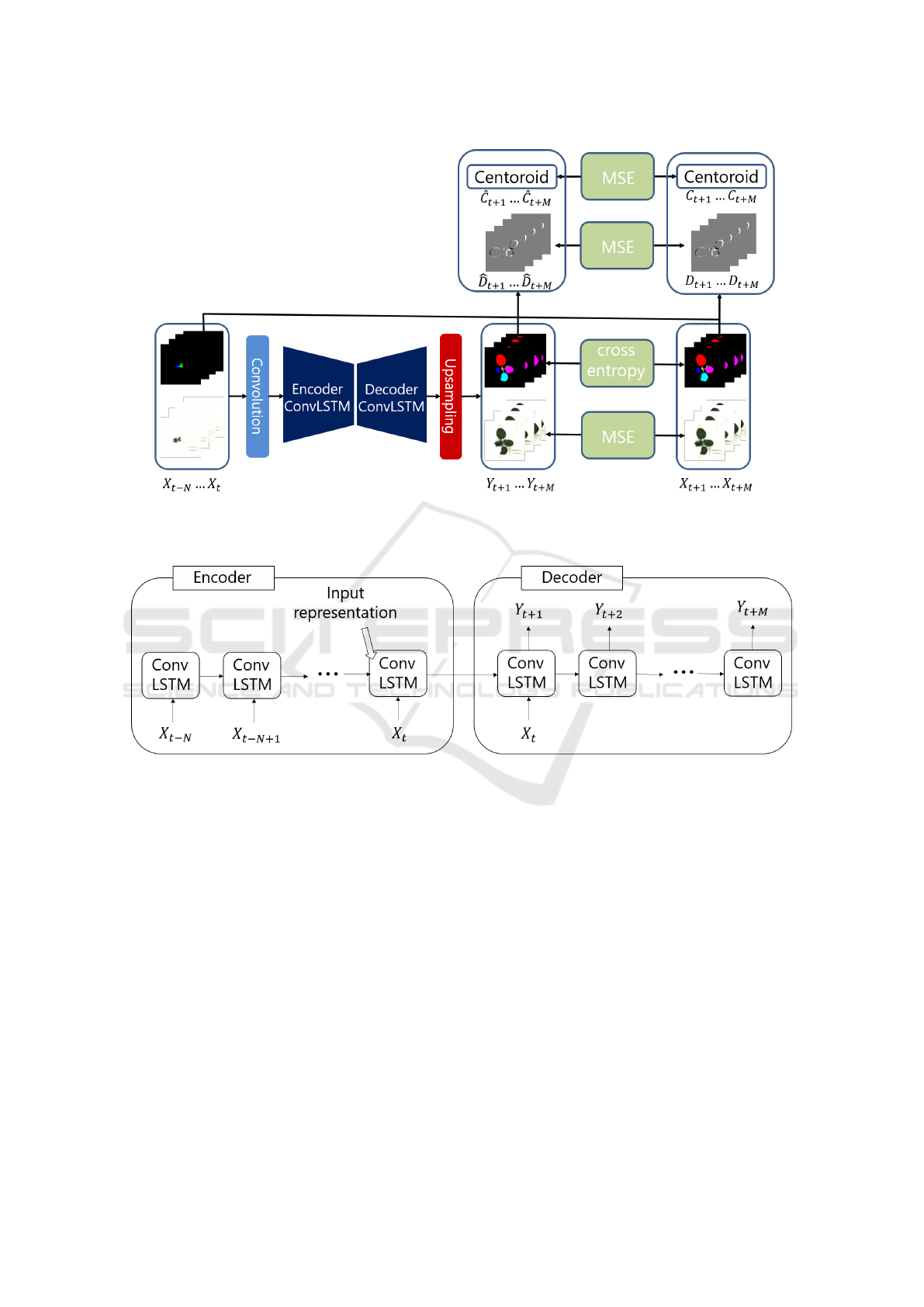
Figure 1: Overview of our proposed network plant growth prediction. Inputs and outputs are a sequence of RGB and labeled
leaf images. Difference images and centroids for the training are obtained from labeled leaf images. Predictions are optimized
by MSE and multi class cross entropy.
Figure 2: Detail of encoder-decoder ConvLSTM structure. The Encoder constructs the representation of inputs over time-steps
and the Decoder predicts time-series future images by the representation.
function of optical flow as a constraint on motion (Liu
et al., 2018). However, as mentioned above, opti-
cal flow is not available in plant growth data due to
large leaf movement. To add constraint of growth ex-
pressly, we propose a difference loss that optimizes
the difference between Y
t
and Y
t−1
. From the experi-
ments, we found that this loss had a role to optimize
expansion of leaves. The difference image of the t-th
frame prediction
ˆ
D
t
and corresponding ground truth
D
t
are defined as follows.
D
t
= X
label
t
− X
label
t−1
(3)
ˆ
D
t
= Y
label
t
−Y
label
t−1
(4)
If there is no previous prediction Y
label
t−1
, X
label
t−1
is used
instead of the prediction. The difference loss L
di f f
is
defined as follows.
L
di f f
(X
t
, Y
t
) = MSE(D
t
,
ˆ
D
t
) (5)
3.4 Centroid Loss
In addition to the difference loss as a constraint of
leaf appearance, we propose to use the centroid loss.
This is designed as a constraint of leaf traits, which
is specific for plant images. Whereas the difference
loss has a role to optimize expansion of leaves, the
centroid loss is has a role to optimize the movement
of leaves. The centroid loss is defined by the centroid
of leaves C
t
and predicted
ˆ
C
t
as follows.
L
cr
(X
t
, Y
t
) = MSE(C
t
,
ˆ
C
t
) (6)
We compute the centroid of leaves using image mo-
ments of labeled leaf images.
VISAPP 2019 - 14th International Conference on Computer Vision Theory and Applications
108

3.5 All Objective Loss
We concatenate all above described loss functions as
a total objective loss. The objective loss is defined as
follows.
L (X
t
, Y
t
) = λ
rgb
L
rgb
(X
t
, Y
t
) + λ
label
L
label
(X
t
, Y
t
)
+λ
di f f
L
di f f
(X
t
, Y
t
) + λ
cr
L
cr
(X
t
, Y
t
)
(7)
We set weights of each loss λ
rgb
, λ
label
, λ
di f f
, λ
cr
as
1.0, 1.0, 2.0, 0.5 respectively.
4 EXPERIMENTS
As described in the previous section, we proposed
two additional loss functions to put constraints on the
change between frames in the plant growth prediction
task. In this section, we evaluate the effectiveness of
our proposed loss functions for the plant growth pre-
diction by using KOMATSUNA dataset (Uchiyama
et al., 2017). As a quantitative evaluation score, we
use the weighted coverage score (Hoiem et al., 2011;
Silberman et al., 2014) between a predicted plant
image result and its ground truth. The detail of the
weighted coverage score is described in Section 4.3.
Also, we visualized prediction of grown plant appea-
rances as a qualitative evaluation.
4.1 Dataset
We used the KOMASTUNA dataset for evaluating
our proposed network because leaf labeling over se-
quence was carefully performed. This dataset con-
tains 5 plants (Komatsuna) sequential data. Each
plant data consists of 60 frames captured every 4
hours from 3 viewpoints. In the experiments, we used
labeled leaf images in addition to RGB images be-
cause we assume that leaf segmentation is done be-
forehand (Ren and Zemel, 2017; Long et al., 2015;
Sakurai et al., 2018a; Li et al., 2016) and its result is
used for the plant growth prediction.
The same label is assigned to each leaf through
both all the frames and all the viewpoint. This label
corresponds to the order of new leaves. In the dataset,
the max leaf label is 8.
For the experiments, we split the data into a trai-
ning dataset and a test one. We used four plant data
for the training and the rest (one plant) for the testing.
We used 128 × 128 image resolution, and augmented
the data with 90, 180 and 270 degrees rotations.
4.2 Training Conditions
4.2.1 Overall Settings
The training dataset has 60 frames. In the experi-
ments, we split 8 frames from the training dataset as
randomly-selected inputs in each iteration for training
the network. This means that it was set that N = 7
and M = 8 in Figure 1. The time of capturing 8 fra-
mes corresponds to 32 hours. However, we did not
use last 8 frames as inputs for the training. If last 8
frames are contained inputs, ground truth correspon-
ding the prediction does not exist. In total, we had
45 sequence of inputs in each dataset. 45 is calcula-
ted by excluding last 8 frames and first 7 frames for
convenience of indices of frames.
In the training process, we applied dropout (Sri-
vastava et al., 2014; Gal and Ghahramani, 2016) to
the ConvLSTM. The dropout rate was set to 0.5.
We used ReLU (Nair and Hinton, 2010) as an acti-
vation function in the prediction network excluding
the ConvLSTM. The activation function of the Con-
vLSTM was hyperbolic tangent (tanh). We used
Adam (Kingma and Ba, 2014) based optimization
with the learning rate α = 0.0001,β1 = 0.5, and β2 =
0.99. This training optimization was iterated 100000
times by using random 8 batches in each iteration.
4.2.2 Network Details
In this section, we explain the detail of the parameters
in the network in Table 1. Conv2D means convolu-
tional layers with 2D filters. Stack means the conca-
tenation of each image along the sequential axis, and
unstack means splitting along the sequential axis.
4.3 Weighted Coverage Score
As described before, we used labeled leaf images for
the evaluation. Thus, the quantitative evaluation was
performed for the predictions of labeled leaf images.
To evaluate predictions, we employ the weighted co-
verage score as an evaluation metric. The weighted
coverage score is computed from the overlap rate be-
tween predictions and ground truth, and the rate is
weighted by the area (the number of pixels) of ground
truth. The weighted coverage score (WCS) is defined
as follows.
WCS(X , Y ) =
1
∑
i
|X
i
|
∑
i
|X
i
|Overlap(X
label
t
, Y
label
t
) (8)
|X
i
| denotes the number of pixels of ground truth and
Overlap(·) means intersection over union (IoU) of
between inputs.
Plant Growth Prediction using Convolutional LSTM
109

Table 1: Parameters of prediction network. When layer is convolutional layer, shape shows filters size. When layer is images,
shape shows images size. Branches are shown right side of the table.
layer shape layer shape
Input (label) 128×128×9 Input (RGB) 128×128×3
Conv2D 3×3×32 Conv2D 3×3×32
Conv2D 4×4×32 2strides Conv2D 4×4×32 2strides
Conv2D 3×3×64 Conv2D 3×3×64
Conv2D 4×4×64 2strides Conv2D 4×4×64 2strides
Concat RGB with label 32×32×128
Stack 8×32×32×128
ConvLSTM(Enc) 3×3×128
ConvLSTM(Dec) 3×3×128
Unstack 32×32×128
Conv2D 3×3×64
Conv2D 4×4×64
Upsampling 64×64×64
Conv2D 3×3×32
Conv2D 4×4×32
Upsampling 128×128×32
Conv2D 3×3×32 Conv2D 3×3×32
Conv2D 3×3×9 Conv2D 3×3×3
Softmax tanh
Output(label) 128×128×9 Output(RGB) 128×128×3
4.4 Results
To evaluate the effectiveness of our proposed diffe-
rence loss and centroid loss for the plant growth pre-
diction, we compared results of the experiment with
or without each loss function. We had four conditi-
ons.
1. No Additional : without both difference loss and
centroid loss
2. Difference : with difference loss and without cen-
troid loss
3. Centroid : without difference loss and with cen-
troid loss
4. Difference+Centroid : with both difference loss
and centroid loss
4.4.1 Quantitative Results
We compared the weighted coverage scores of all the
results of each condition described in Table 2. The
leaf labels in KOMATSUNA dataset included 1 to 8
excluding background. However, the number of trai-
ning data including 8 labeled leaves is few and the
score is 0 in all conditions. Thus we excluded the
score of leaf8 from this table and the following re-
sults.
Table 2 shows the coverage score with the additi-
onal loss function tended to decrease for leaves of the
earlier stage but increase for leaves of the later stage.
In the earlier stage, leaves were small and shew little
change between frames. On the other hand, in the
later stage, leaves were large and shew great change
between frames. In terms of the purpose to optimize
the change for the plant growth prediction, the effecti-
veness of proposed loss functions were shown. Alt-
hough We could see that difference loss was more ef-
fective than centroid loss, uniting difference loss with
centroid loss showed the best score in many leaves
containing mean coverage score.
4.4.2 Qualitative Results
Figure 3 shows the prediction of labeled leaf images
Y
label
in each condition and its ground truth X
label
.
Figure 4 shows the rgb images Y
rgb
and X
rgb
. We
can see the prediction error in yellow leaves in results
of No Additional. Such type of error disappeared by
adding proposed loss. This shows proposed loss im-
proved the visual quality of prediction. Indeed, re-
sults employed both loss function were more consis-
tent than any other results. In prediction of RGB ima-
ges, shape of leaves roughly same with corresponding
labeled leaf images but all results are blurred. To im-
prove the sharpness of rgb images, other strategy was
required.
VISAPP 2019 - 14th International Conference on Computer Vision Theory and Applications
110
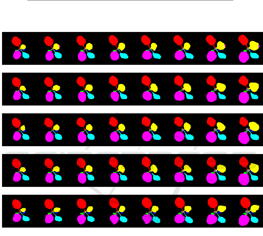
Table 2: Weighted coverage score of experimental result on KOMATSUNA dataset. Rows show score of each leaf prediction
and mean over leaves. Colomns show condition of loss function.
leaf1 leaf2 leaf3 leaf4 leaf5 leaf6 leaf7 mCov
No Additional Loss 72.5 68.7 67.8 72.6 66.6 61.1 32.4 67.2
Difference 72.1 67.1 67.2 73.4 69.2 60.7 37.5 67.9
Centroid 71.8 65.2 68.5 72.7 67.7 59.5 34.8 67.1
Difference+Centroid 72.8 64.7 68.2 74.3 69.0 62.2 37.2 68.1
(a) No Additional
(b) Difference
(c) Centroid
(d) Difference+Centroid
(e) Ground Truth
Figure 3: Predicted results of label images. Leftmost is the first frame and rightmost is the last frame. (a)-(d) show result of
prediction and (e) shows its ground truth.
5 CONCLUSION
In this paper, we proposed the plant growth pre-
diction network inspired by the future frame pre-
diction and loss functions to optimize change of le-
aves between frames. We compared several conditi-
ons with/without proposed loss functions and evalu-
ated results by the weighted coverage score of each
leaf as the quantitative evaluation and the predicted
appearance as the qualitative evaluation. Uniting both
difference loss and centroid loss showed higher per-
formance than the condition with no additional loss
and gave the effectiveness to constrain the change of
leaves.
ACKNOWLEDGEMENT
A part of this research was funded by JSPS KA-
KENHI grant number JP17H01768 and JP18H04117.
Plant Growth Prediction using Convolutional LSTM
111
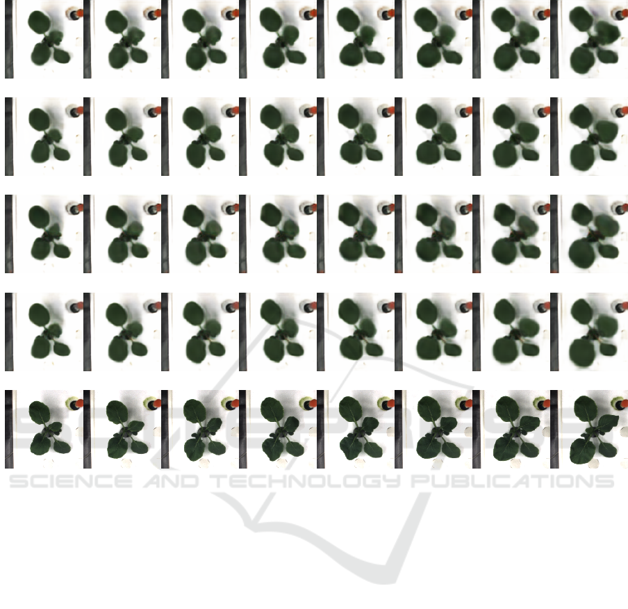
(a) No Additional
(b) Difference
(c) Centroid
(d) Difference+Centroid
(e) Ground Truth
Figure 4: Leftmost is the first frame and rightmost is the last frame. (a)-(d) show result of prediction and (e) shows its ground
truth.
REFERENCES
Barbagallo, R. P., Oxborough, K., Pallett, K. E., and Ba-
ker, N. R. (2003). Rapid, noninvasive screening for
perturbations of metabolism and plant growth using
chlorophyll fluorescence imaging. Plant Physiology,
132(2):485–493.
Gal, Y. and Ghahramani, Z. (2016). A theoretically groun-
ded application of dropout in recurrent neural net-
works. In Advances in neural information processing
systems, pages 1019–1027.
Goodfellow, I., Pouget-Abadie, J., Mirza, M., Xu, B.,
Warde-Farley, D., Ozair, S., Courville, A., and Ben-
gio, Y. (2014). Generative adversarial nets. In Advan-
ces in neural information processing systems, pages
2672–2680.
Hochreiter, S. and Schmidhuber, J. (1997). Long short-term
memory. Neural computation, 9(8):1735–1780.
Hoiem, D., Efros, A. A., and Hebert, M. (2011). Recovering
occlusion boundaries from an image. International
Journal of Computer Vision, 91(3):328–346.
Kingma, D. P. and Ba, J. L. (2014). Adam: Amethod for
stochastic optimization. In Proc. 3rd Int. Conf. Learn.
Representations.
Ledig, C., Theis, L., Huszar, F., Caballero, J., Cunningham,
A., Acosta, A., Aitken, A., Tejani, A., Totz, J., Wang,
Z., et al. (2017). Photo-realistic single image super-
resolution using a generative adversarial network. In
Proceedings of the IEEE Conference on Computer Vi-
sion and Pattern Recognition, pages 4681–4690.
Li, K., Hariharan, B., and Malik, J. (2016). Iterative in-
stance segmentation. In The IEEE Conference on
Computer Vision and Pattern Recognition (CVPR).
Li, L., Zhang, Q., and Huang, D. (2014). A review of
imaging techniques for plant phenotyping. Sensors,
14(11):20078–20111.
Liu, W., Luo, W., Lian, D., and Gao, S. (2018). Future
frame prediction for anomaly detection a new base-
line. In The IEEE Conference on Computer Vision
and Pattern Recognition (CVPR).
Long, J., Shelhamer, E., and Darrell, T. (2015). Fully con-
volutional networks for semantic segmentation. In
VISAPP 2019 - 14th International Conference on Computer Vision Theory and Applications
112

Proceedings of the IEEE conference on computer vi-
sion and pattern recognition, pages 3431–3440.
Luc, P., Couprie, C., Chintala, S., and Verbeek, J. (2016).
Semantic segmentation using adversarial networks. In
NIPS Workshop on Adversarial Training.
Mathieu, M., Couprie, C., and LeCun, Y. (2016). Deep
multi-scale video prediction beyond mean square er-
ror. ICLR.
Moriyuki, S. and Fukuda, H. (2016). High-throughput gro-
wth prediction for lactuca sativa l. seedlings using
chlorophyll fluorescence in a plant factory with arti-
ficial lighting. Frontiers in plant science, 7:394.
Nair, V. and Hinton, G. E. (2010). Rectified linear units im-
prove restricted boltzmann machines. In Proceedings
of the 27th international conference on machine lear-
ning (ICML-10), pages 807–814.
Ranzato, M., Szlam, A., Bruna, J., Mathieu, M., Collo-
bert, R., and Chopra, S. (2014). Video (language)
modeling: a baseline for generative models of natu-
ral videos. CoRR, abs/1412.6604.
Ren, M. and Zemel, R. S. (2017). End-to-end instance seg-
mentation with recurrent attention. In Proceedings of
the 2017 IEEE Conference on Computer Vision and
Pattern Recognition (CVPR), Honolulu, HI, USA, pa-
ges 21–26.
Sakurai, S., Uchiyama, H., Shimada, A., Arita, D., and
ichiro Taniguchi, R. (2018a). Two-step transfer le-
arning for semantic plant segmentation. In Procee-
dings of the 7th International Conference on Pattern
Recognition Applications and Methods - Volume 1:
ICPRAM,, pages 332–339. INSTICC, SciTePress.
Sakurai, S., Uchiyama, H., Shimada, A., Arita, D., and Ta-
niguchi, R. (2018b). Two-step transfer learning for se-
mantic plant segmentation. In 7th International Con-
ference on Pattern Recognition Applications and Met-
hods (ICPRAM2018).
Silberman, N., Sontag, D., and Fergus, R. (2014). Instance
segmentation of indoor scenes using a coverage loss.
In European Conference on Computer Vision, pages
616–631. Springer.
Srivastava, N., Hinton, G., Krizhevsky, A., Sutskever, I.,
and Salakhutdinov, R. (2014). Dropout: A simple way
to prevent neural networks from overfitting. The Jour-
nal of Machine Learning Research, 15(1):1929–1958.
Srivastava, N., Mansimov, E., and Salakhudinov, R. (2015).
Unsupervised learning of video representations using
lstms. In International conference on machine lear-
ning, pages 843–852.
Sutskever, I., Vinyals, O., and Le, Q. V. (2014). Sequence
to sequence learning with neural networks. In Advan-
ces in neural information processing systems, pages
3104–3112.
Ubbens, J. R. and Stavness, I. (2017). Deep plant pheno-
mics: a deep learning platform for complex plant phe-
notyping tasks. Frontiers in plant science, 8:1190.
Uchiyama, H., Sakurai, S., Mishima, M., Arita, D., Oka-
yasu, T., Shimada, A., and Taniguchi, R.-i. (2017).
An easy-to-setup 3d phenotyping platform for komat-
suna dataset. In The IEEE International Conference
on Computer Vision (ICCV) Workshops.
Villegas, R., Yang, J., Hong, S., Lin, X., and Lee, H. (2017).
Decomposing motion and content for natural video se-
quence prediction. ICLR.
Walter, A., Liebisch, F., and Hund, A. (2015). Plant
phenotyping: from bean weighing to image analysis.
Plant methods, 11(1):14.
Xingjian, S., Chen, Z., Wang, H., Yeung, D.-Y., Wong, W.-
K., and Woo, W.-c. (2015). Convolutional lstm net-
work: A machine learning approach for precipitation
nowcasting. In Advances in neural information pro-
cessing systems, pages 802–810.
Zaidi, M., Murase, H., and Honami, N. (1999). Neural net-
work model for the evaluation of lettuce plant gro-
wth. Journal of agricultural engineering research,
74(3):237–242.
Plant Growth Prediction using Convolutional LSTM
113
