
Maximization of Profit for a
Problem of Location and Routing, with Price-sensitive Demands
Narda E. Ibarra-Delgado
1
, Elias Olivares-Benitez
1
, Samuel Nucamendi-Guillén
1
and Omar G. Rojas
2
1
Universidad Panamericana, Facultad de Ingenieria, Prolongacion Calzada Circunvalacion Poniente 49, Zapopan,
Jalisco, 45010, Mexico
2
Universidad Panamericana, Escuela de Ciencias Económicas y Empresariales
Prolongacion Calzada Circunvalacion Poniente 49, Zapopan, Jalisco, 45010, Mexico
Keywords: Location Routing Problem, Price-sensitive Demand, Heuristic.
Abstract: This article seeks to study and solve a problem of profit maximization of a company by defining the location
of an optimal number of facilities, allocation and routing of vehicles, and costs for home delivery to meet the
demand of its customers. This study is based on an article in which, for the first time, a problem of location
and routing and maximization of utilities with price-sensitive demands is integrated. This problem, unlike
other studies that only minimize other metrics such as waiting times, route distances, and transportation costs,
seeks a greater benefit by increasing profits by discriminating prices depending on the customer's location or
adding an additional cost to retail sales. This paper presents a model for small instances based on the model
proposed in the aforementioned article. Next, a two-phase heuristic is proposed that solves larger instances
with a result close to that obtained in the previous article where a branch-and-price heuristic was used.
1 INTRODUCTION
In problems of transport and distribution, there are
cases where decisions must be made that affect the
supply chain in the long term, in the short term and
daily; these are called strategic, tactical and
operational decisions, respectively (Fazayeli et al.,
2017). The location and routing problem (LRP)
includes two types of problems fundamental to supply
chain management: the problem of facility location of
and the problem of vehicle routing. Because both
problems are related, LRP problems have recently
become an interesting area of study (Archetti et al.,
2017).
The classic problems of location and routing,
where a set of potential distribution centers, opening
costs, identical vehicles and a set of known demands
are defined, consist of selecting which distribution
centers will be opened, assigning customers and
determining the route of each available vehicle. The
objective is to minimize the total cost, which includes
the cost of opening each center, the fixed cost of the
vehicles and the total cost of transportation (Prodhon
and Prins, 2014). Panicker et al. (2018) solve a
location-routing problem using an ant-colony
optimization heuristic, for instances generated by the
authors. Ferreira and Alves de Queiroz (2018) solve
a LRP using heuristics based on simulated annealing
with good results for instances of up to 200
customers.
There are several extensions to the Location-
Routing Problem in the literature. Sarham et al.
(2018) developed a column-generation approach to
solve the LRP with time windows. Chen et al. (2018)
investigate a LRP with full truckloads for designing a
low-carbon supply chain. They developed a hybrid
heuristic combining NSGA-II and Tabu Search. Guo
et al. (2018) study a closed-loop supply chain where
location, inventory, and routing decisions must be
made. They propose the mathematical model and
develop a hybrid heuristic that combines simulated
annealing and genetic algorithms to solve several
instances.
Ahmadi-Javid et al. (2018) studied a problem that,
unlike the classic problems of location and routing,
besides minimizing costs, seeks to maximize profits
managing delivery costs considering the demand and
location of the customers. However, due to the
complexity of this situation, in addition to proposing
a mixed integer linear model (MILP), the authors
developed a branch-and-price heuristic to obtain a
feasible solution for large instances.
414
Ibarra-Delgado, N., Olivares-Benitez, E., Nucamendi-Guillén, S. and Rojas, O.
Maximization of Profit for a Problem of Location and Routing, with Price-sensitive Demands.
DOI: 10.5220/0007405304140421
In Proceedings of the 8th International Conference on Operations Research and Enterprise Systems (ICORES 2019), pages 414-421
ISBN: 978-989-758-352-0
Copyright
c
2019 by SCITEPRESS – Science and Technology Publications, Lda. All rights reserved

For this study, an alternate two-phase heuristic is
presented to solve the problem proposed by Ahmadi-
Javid et al. (2018). The heuristic consists of pre-
grouping the customers, and assigning to the nearest
centers to create small instances that can be solved
with the MILP model. Despite its simplicity, this
heuristic achieves results similar to those obtained
with branch-and-price heuristics.
2 LITERATURE REVIEW
Ahmadi-Javid et al. (2018) made reference to Laporte
(Albareda-Sambola et al., 2007), who has contributed
to the study of this problem with different
formulations, solution methods and computational
results, as well as other authors (Nagy and Salhi,
2007; Borges Lopes et al., 2013). In addition, they
mentioned recent investigations of variants of this
model, such as a model for a stochastic supply chain
system (Ahmadi-Javid and Azad, 2010) and a
location and routing model with production and
distribution with risks of interruption in a supply
chain network (Ahmadi-Javid and Seddighi, 2013).
In most cases, the problems of location and
routing establish that all customers must be visited
and their demands must be met (Ahmadi-Javid et al.,
2018). However, the problem seeks to maximize the
total utility, minimizing the cost of transportation and
the cost of establishing distribution centers without
necessarily having to attend to all their potential
customers. Likewise, there are other articles (Nagy
and Salhi, 1998), where it is allowed to visit the
customer more than once, others where some do not
need to be visited (Averbakh and Berman, 1994;
1995), and others where some randomly selected
customers are not visited (Albareda-Sambola et al.,
2007). This is because sometimes the cost exceeds the
income generated by serving them.
Although the model of Ahmadi-Javid et al.
(2018) is one of the few investigations on problems
of location and routing with multi-objectives, there
are other similar models such as the Traveling
Salesman Problem (TSP) or Vehicle Routing
Problem (VRP), which are among the most studied
combinatorial optimization problems. In addition,
there are extensions of these that make decisions
based on the profits generated by visiting only certain
customers, such as in the case of the traveler with
profit (TSPPs), or the problem of vehicle routing with
profits (VRPPs).
Of the previously mentioned models, the one
that most resembles maximization of profit for a
problem of location and routing (Ahmadi-Javid et al.,
2018) is the problem of vehicle routing with profits.
Unlike the classic problems, the customers that will
be attended must be selected, since the set is not
defined, and the route in which these customers will
be served, taking into account how attractive the
customer is for the profit that can generate (Archetti
and Speranza, 2014).
However, in this case of routing with profits,
only one distribution center is available. The problem
of routing vehicles with multiple deposits is a
variation of VRP, which has the same objectives.
However, it has several vehicles and potential
distribution centers (Archetti et al., 2014). Aras et al.
(2011) presented a selective model of vehicle routing
with multiple deposits and prices, where only those
customers that are profitable are served.
Another particularity of the model proposed by
Ahmadi-Javid et al. (2018) is that the known demand
of each customer changes according to the assigned
price. They mention that price sensitive demand has
been integrated into different models. However, it is
the first time that sensitive demands are taken into
account for a location and routing problem.
In addition, they mention that the model most
similar to theirs is that of Archetti et al. (2014) who
solve a VRP with profits, which consists of
maximizing the difference of the obtained profits and
the cost of transport, using a single distribution center
and a fleet of identical vehicles. Unlike the study by
Archetti et al. (2014), they model a problem with the
same objectives, but with several potential
distribution centers and with price sensitive demands,
making their problem more complex since each
center can offer different prices to each customer.
3 PROBLEM DESCRIPTION AND
MATHEMATICAL MODEL
In this Profit-Maximization Location-Routing
Problem (PM-LRP), we have a set of possible
locations for distribution centers, with equal capacity
and a set of locations for potential customers with
their respective initial demands. Also, a number of
available vehicles with equal capacity is defined. The
objective is to maximize profits, minimizing the total
cost of opening centers and transport. To achieve this,
it is necessary to determine which centers to open,
which customers to assign to each center with the
possibility of not attending to all, the prices assigned
to each customer taking into account the variation in
demand based on the price assigned, the vehicles to
each distribution center, and the route of each vehicle
Maximization of Profit for a Problem of Location and Routing, with Price-sensitive Demands
415

by visiting the selected customers only once.
To decide the delivery prices for each customer,
Ahmadi-Javid et al. (2018) use a space price policy,
which consists of assigning an equal retail price for
all customers adding an additional cost depending on
their location. This added cost per delivery is an
additional percentage of the retail price, which is
called markup. For this model 6 or 11 levels of
markup are used depending on the instance ranging
from the percentages
0.1 to 0.2, in intervals of 0.1
for the instances of 6 markups, or in intervals of 0.05
for instances of 11 Markups. Therefore, the pricing
decision is to define the level of markup to add to
overall price considering that initial claims assigned
vary depending on the final price. This final price
is called the delivery price. This is a type of price
discrimination that can only be applied if the exact
location of the potential customers is known, and is
given by
, where is the retail
price, and
the extra percentage at the level of
markup . For the demands to be modified depending
on the final price, the following negative slope
function was used (Greenhut et al., 1975):
,
< a / b
Where d
il
is the final demand of customer i with the
level of markup l,
the end price of the product with
the markup level l, and a, b and v are positive
parameters which for this model were established as
10.1, 1.5, and 0.25, respectively.
Mathematical model proposed by Ahamid-Javid et al.
(2018)
Sets
Set of potential customers
Set of potential distribution centers
Set of markup levels
Set of Available Vehicles
Auxiliary Sets
Set of all possible nodes (Distribution centers
and customers), i.e.,
Set of virtual vehicles assigned to the
distribution center
,i.e.
Parameters
Distance from node i to node j,
Fixed cost per unit of distance
Vehicle capacity, same for all vehicles
Capacity of Distribution Center
Base price of the product
Percentage associated with the level of
markup l
Delivery price per unit of product associated
with the markup level l, which is obtained
by
The demand of the customer i to which the
extra percentage of the level is charged
markup l,
Fixed cost of establishing a distribution center
The distribution center to which the vehicle
k
is assigned, i.e.,
Decision Variables
Binary variable that becomes 1 if node j is
visited just after node i by vehicle k, or 0
otherwise,
Binary variable that becomes 1 if node i is
visited by vehicle k with the markup level l
Binary variable that is used, 1 if distribution
center h is selected to be set or 0 otherwise. ,
Non-negative auxiliary for customer i used in
MTZ sub-tour elimination constraint of the
virtual path of
Objective Function
Maximize:
(1)
Subject to
(2)
(3)
(4)
(5)
(6)
(7)
(8)
(9)
ICORES 2019 - 8th International Conference on Operations Research and Enterprise Systems
416

(10)
(11)
(12)
(13)
The objective (1) is to maximize the profit, which is
the profit generated by serving customers minus the
cost of establishing the distribution centers and the
cost of transportation of the routes. Restrictions (2)
ensure that each customer can only be visited once.
Restrictions (3) define that the times a vehicle enters
a distribution center is equal to the times it leaves it.
Restrictions (4) ensure that each vehicle can only
make one route. Restrictions (5) determine the
connectivity of each route by determining the
assignment of customers to each vehicle. Restrictions
(6) limit the capacity of the vehicles and (7) ensure
that the demand covered by each distribution center
does not exceed its capacity. Restriction (8) limits the
number of vehicles available. Restrictions (9) and
(10), are Miller-Tucker-Zemlin sub-tour elimination
constraints published by Miller et al. (1960), and
restrictions (11-13) make the decision variables
binary.
4 SOLUTION METHODS
Ahmadi-Javid et al. (2018), proposed the MILP
model of polynomial size previously described to be
able to solve small instances. This was programmed
in CPLEX 12.3. Several major instances were run
which were stopped after a few hours in order to
obtain a feasible result, although the global optimum
was not reached. To improve these results, Ahmadi-
Javid et al. (2018), proposed a branch-and-price
heuristic by previously creating an exponential size
formulation of grouped sets using the decomposition
of Dantzig-Wolfe, which simplifies the problem by
dividing it into a master problem and several sub-
problems. This model was programmed in C++.
4.1 Heuristic
As an alternative to solving this problem, a two-phase
heuristic is proposed that aims to create sub-problems
to decrease and divide the number of variables and
restrictions in each phase. Previously, the MILP was
programmed in LINGO to be able to verify the correct
interpretation.
4.1.1 First Phase
The first phase consists of creating routes with the
minimum possible demand, that is, with the highest
level of markup taking into account the capacity
restriction of each vehicle and distribution centers,
but without taking into account the number of
vehicles available. This phase is started by selecting
the distribution center with the lowest sum of the
distance between the nearest potential customers.
Starting with the previously selected distribution
center, a subgroup is created using the nearest
neighbor algorithm. The stopping criterion for the
heuristic of the nearest neighbor is executed when the
sum of the minimum demands (markup 6 or 11) of the
selected customers exceeds the capacity of the vehicle
of that route, or the capacity of the distribution center
taking account the demand covered by the routes
previously assigned to that center.
Then the previously created group is taken to run
a small instance with the MILP model, where it is
established that only one vehicle is available to obtain
a route. Due to the small number of variables, there is
an optimal global solution for that combination,
selecting the best route and the level of markup for
each customer. Since the model in MILP is
programmed to serve only those customers that are
profitable, the customers that are not part of the result
are taken into account for the pre-grouping of another
possible route and the others that were assigned are
eliminated. The creation of possible routes ends when
all customers have been assigned to some route, when
the capacities of all the distribution centers are to be
exceeded by the sum of covered demands of the
routes assigned to them, or when there are no longer
profitable customers to attend.
Input data for the first phase:
Set of potential customers ;
coordinate x, coordinate y, initial
demand
Set of Distribution Centers
coordinate x, coordinate y
Capacity of vehicles
Capacity of distribution centers
No. of markup levels = 611}
Calculations for the first phase:
1. Distancesbetween all possible nodes ϵ
These distances are calculated with the
Euclidean formula.
Maximization of Profit for a Problem of Location and Routing, with Price-sensitive Demands
417

(14)
2. Adjusted demands of all customers for all
markup levels ,
110 15 025
(15)
3. Profit to cover customer demand in the
mark up
(16)
4. Maximum number of customers to take into
account for possible routes
(17)
PHASE 1. HEURISTICS-CREATION OF ROUTES
START
Input: set customers, set distribution centers, vehicle
capacity, capacity distribution centers, initial demand,
markup levels set
r = 1
Do Until | I | = 0 or | H | = 0
1. Select distribution center using selection
procedure Fig. 2
2. Create subgroup using subgroup creation
procedure Fig.3
3. Solve MILP model, according to equations 1-13,
with data from subgroup to generate r, with a
single vehicle k
4. IF profit of r = 0, delete selected center h from
H, return to step 1.
5.
selected =
selected- demand covered in route
6. IF belongs to solution r, eliminate
7. r=r+1
LOOP
Output: set of routes R, profit of routes
Figure 1: Heuristic- creation of routes.
SELECTION PROCEDURE DISTRIBUTION
CENTER
Input: coordinates set | I |, coordinates set | H |, Q
START
1. Calculate Euclidean distances of
according to equation (14).
2. IF Q (eq. 17) |I|, THEN add distances of Q
nearest customers to ,
ELSE add all distances.
3. Select the center with the shortest distance
added in step 2.
Output: Selected center
END
Figure 2: Selection procedure for distribution centers.
SUBGROUP CREATION PROCEDURE
Input: coordinates set | I |, coordinates selected center,
initial demand | I |, demand at mark level -up greater for
set | I |, capacity distribution center selected
Accumulated capacity = 0
START
1) IF
selected ,
THEN =
selected
DO WHILE ℎ selected <accumulated
capacity
1) Create selected center distance matrix a
2) Starting at selected center, select nearest
neighbor according to algorithm.
3) Add nearest neighbor to subgroup
4) Cumulative demand = cumulative demand +
demand at the higher markup level of nearest
neighbor from step 4 according to equation (15).
LOOP
END
Output: subgroup set
Figure 3: Subgroup creation procedure.
4.1.2 Second Phase
The second phase consists of a model that aims to
maximize the profit by selecting routes created in
phase 1 of the set having as the sole restriction the
number of vehicles available. The other restrictions of
the problem are taken into account for the creation of
said routes and subtracting the opening cost of each
center if at least one route is selected in said center.
This problem contains disjunctive constraints, since
the binary variable that multiplies the cost of
establishing a center takes the value of 1 when there
ICORES 2019 - 8th International Conference on Operations Research and Enterprise Systems
418
is at least one selected route from that distribution
center as shown in the constraint (20). The second
phase was solved using Excel solver.
Input data for second phase:
Set of possible routes assigned to
Set of distribution centers
Available vehicles
profit of each route
Fixed cost of establishing distribution centers
Model Phase 2
From the output of phase 1 (Fig 1.) the following
model is solved:
1
1
;
(18)
Subject to
(19)
=
(20)
(21)
(22)
The objective (18) is to maximize the total profit;
that is, the profit of the selected routes minus the cost
to open the distribution centers. Restriction (19)
ensures that the accepted number of routes is equal to
the number of vehicles available. Restriction (20)
gives the value of 1 if at least one route assigned to
the distribution center was accepted, or 0 if
none was accepted. Restrictions (21-22) ensure that
the variables of accepting a route and opening a
distribution center are binary.
5 EXPERIMENTATION
In the instances used, the number of potential
customers and the number of distribution centers
available are first defined. Then the coordinates in x
and y, and the initial demands of the customers. Then
the capacities of the centers and the cost of
establishing them are presented. Finally, the capacity
of the vehicles, the available number and the cost per
unit of distance are shown. For all instances, the base
price 5 was established. Each instance was
resolved with both levels of markup 6 and 11. To
name the instances, the initial of the author of the
instance was taken, followed by the number of
available customers, the number of distribution
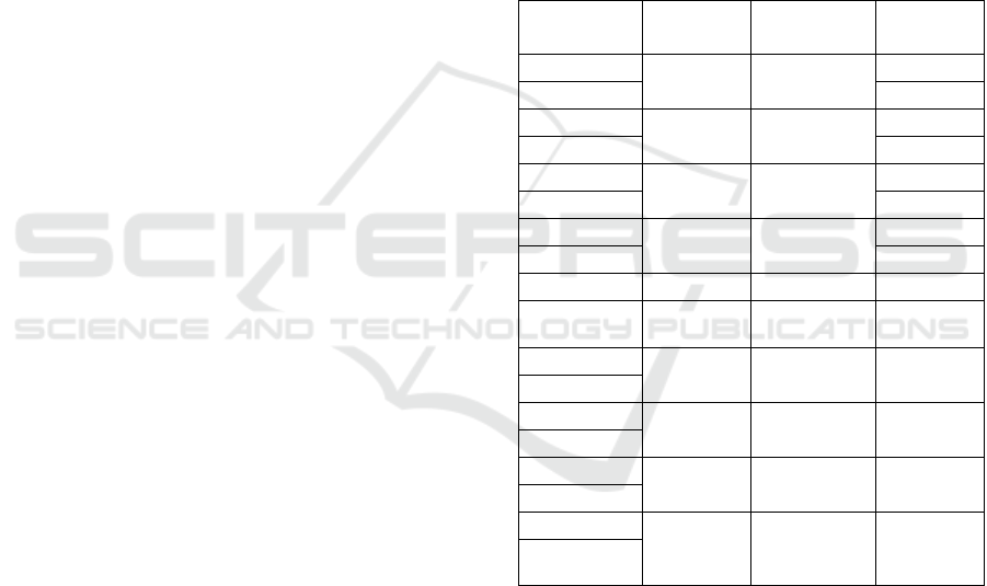
centers and the level of markup. Table 1 shows the
original names of the instances with their respective
data. Since this problem is new, the instances were
generated modifying LRP benchmark instances
available in the literature. The original names of the
instances are shown in Table 1.
Table 1: Instances.
Instance
name
Original
name
no.
customers
mark up
levels
Pe-12x2x6
Perl183-
12-2
12
6
Pe-12x2x11
11
G-21x5x6
Gaskell67
-21x5
21
6
G-21x5x11
11
G-22x5x6
Gaskell67
-22x5
22
6
G-22x5x11
11
M-27x5x6
Min92-
27x5
27
6
M-27x5x11
11
Cap DC
Fixed cost
vehicle
capacity
Pe-12x2x6
280
100
140
Pe-12x2x11
G-21x5x6
15000
50
6000
G-21X5X11
G-22X5X6
15000
50
4500
G-22X5X11
M-27X5X6
9000
272
2500
M-
27X5X11
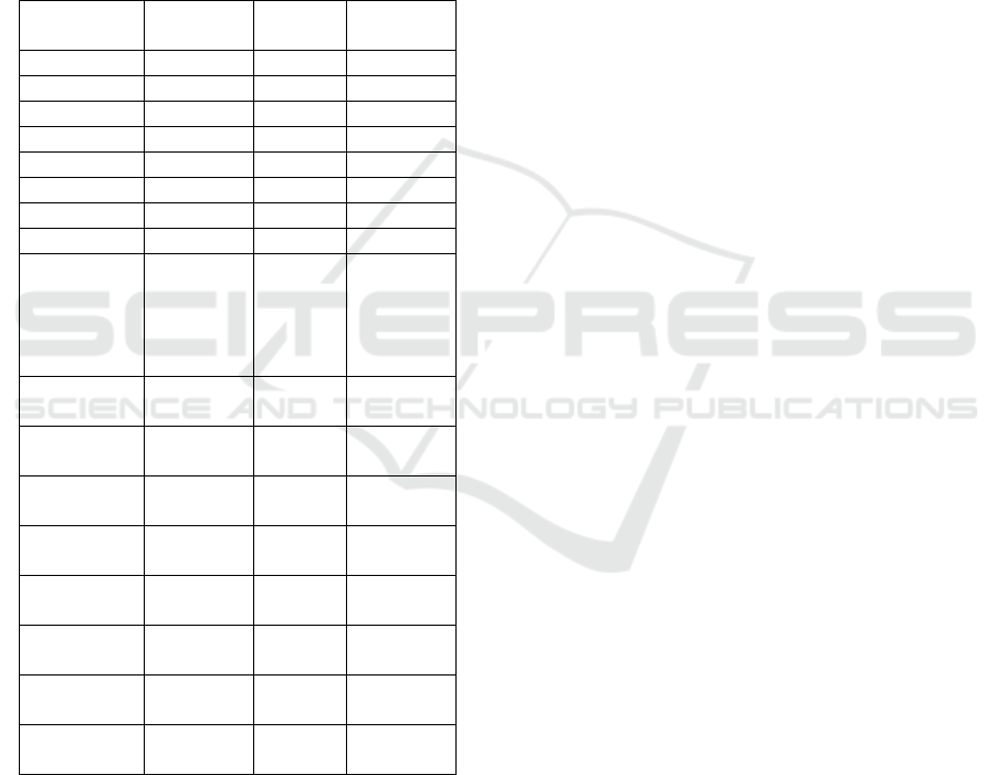
6 RESULTS
Table 2 summarizes the best solution of the objective
value, and the number of variables for the eight
instances in the four proven methods: the MILP in
CPLEX, the branch-and-price heuristic by Ahmadi-
Javid et al. (2018), the method in LINGO and the
proposed two-phase heuristic. The last column shows
the error percentage of the two-phase heuristic on the
best solution found among the other methods.
Maximization of Profit for a Problem of Location and Routing, with Price-sensitive Demands
419
For the smallest instance, the program was
allowed to run until finding the global optimum; after
12 hours with 30 minutes, the overall optimum was
obtained, seven hours after the model in CPLEX. In
the results, a difference of 0.60 is shown, which may
be due to decimals considered in each engine used.
For all other instances, a limit of ten hours was
established, and the program was interrupted in Lingo
in order to find a feasible solution. For the two-phase
heuristic it was not possible to measure the time, since
a part was done manually in Excel, and another in
LINGO.
Table 2: Results in objective value.
Instance
name
CPLEX
B & B
ALG
LINGO
Pe-12x2x6
71.08
71.08
71.68
Pe-12x2x11
96.66
96.66
87.9
G-21x5x6
17775.06
17859
17535.97
G-21x5x11
18290.59
18391.9
17595.64
G-22x5x6
8667.44
8927.72
8706.022
G-22x5x11
9097.83
9097.83
8873.885
M-27x5x6
2927.16
2927.16
2633.36
M-27x5x11
3543.58
3543.58
3207.085
TWO
PHASES
NO. OF
VARIA
BLES
%
ERROR
VS. BEST
SOLUTIO
N
Pe-12x2x6
65.28
1181
8.929%
Pe-12x2x11
91.09
1461
5.762%
G-21x5x6
17064.727
17168
4.447%
G-21x5x11
17520.293
19768
4.739%
G-22x5x6
8840.96
18368
0.972%
G-22x5x11
8936.687
21068
1.771%
M-27x5x6
2926.5927
24968
0.019%
M-27x5x11
3492.1874
28168
1.450%
For the percentage of error on the best solution
found with the two-phase heuristic solution, it can be
seen that the greater the number of variables, the
percentage of error tends to decrease, behaving
similarly when you have 6 or 11 associated markup
levels.
On the other hand, the improvement due to
increasing the number of markup levels is positive in
all cases for all the methods used. However, there is
no trend associated with the number of variables but
rather, with another particularity of each instance,
since the smallest instance and the largest one, have a
much more significant increase than the two median-
size instances.
7 CONCLUSIONS
The results of the heuristic were satisfactory.
However, no result was better than that obtained in
the heuristic proposed by Ahmadi-Javid et al. (2018).
In spite of not being able to measure the time for the
metaheuristic, it can be seen that a better result is
obtained than in the MILP. As shown in Table 2, the
percentage of errors decreases as the size of the
instance increases. It may be that this method obtains
better results with larger instances.
As in the reference article, implementing the
differentiation of prices for each customer when the
demands are price sensitive increases significantly to
a greater number of markup levels. That is, this policy
can increase company profits, however, it would be
difficult to predict the behavior of the demands for
each customer, making the problem less feasible for
real cases.
For future research, we will code the heuristic in
C++, in order to compare the execution times.
Moreover, it is expected to analyze the effects of the
sensitivity of the demand in the maximization of
profit, to be able to apply a penalty according to those
customers who should not be served.
ACKNOWLEDGEMENTS
This research was supported by Universidad
Panamericana [grant number UP-CI-2018-ING-
GDL-06].
REFERENCES
Ahmadi-Javid, A, Amiri, E, and Meskar, M, 2018. A Profit-
Maximization Location-Routing-Pricing Problem: A
Branch-and-Price Algorithm. European Journal of
Operational Research, vol. 271, no. 3, pp. 866-881.
Ahmadi Javid, A, and Azad, N, 2010. Incorporating
location, routing and inventory decisions in supply
chain network design. Transportation Research Part E:
Logistics and Transportation Review, vol. 46, no. 5, pp.
582–597.
Ahmadi-Javid, A, and Seddighi, A H, 2013. A location,
ICORES 2019 - 8th International Conference on Operations Research and Enterprise Systems
420

routing problem with disruption risk. Transportation
Research Part E: Logistics and Transportation Review,
vol. 53, pp. 63–82.
Albareda-Sambola, M, Fernández, E, and Laporte, G, 2007.
Heuristic and lower bound for a stochastic location-
routing problem. European Journal of Operational
Research, vol. 179, no. 3, pp. 940–955.
Archetti, C, Bertazzi, L, Laganà, D, and Vocaturo, F, 2017.
The Undirected Capacitated General Routing Problem
with Profits. European Journal of Operational
Research, vol. 257, no. 3, pp. 822–833.
Archetti, C, and Speranza, M G, 2014. A survey on
matheuristics for routing problems. EURO Journal on
Computational Optimization, vol. 2, no. 4, pp. 223–
246.
Archetti, C, Speranza, M G, and Vigo, D, 2014. Vehicle
routing problems with profits. Vehicle Routing:
Problems, Methods, and Applications, 2nd Edition, pp.
273–297.
Averbakh, I, and Berman, O, 1994. Technical Note—
Routing and Location-Routing p-Delivery Men
Problems on a Path. Transportation Science, vol. 28,
no. 2, pp. 162–166.
Averbakh, I, and Berman, O, 1995. Probabilistic Sales-
Delivery Man and Sales-Delivery Facility Location
Problems on a Tree. Transportation Science, vol. 29,
no. 2, pp. 184–197.
Borges Lopes, R, Ferreira, C, Sousa Santos, B, and Barreto,
S, 2013. A taxonomical analysis, current methods and
objectives on location‐routing problems. International
Transactions in Operational Research, vol. 20, no. 6,
pp. 795-822.
Chen, C, Qiu, R, and Hu, X, 2018. The Location-Routing
Problem with Full Truckloads in Low-Carbon Supply
Chain Network Designing. Mathematical Problems in
Engineering, vol. 2018, no. 1, Article ID 6315631, 13
pages.
Fazayeli, S, Eydi, A, and Kamalabadi, I N, 2017. A model
for distribution centers location-routing problem on a
multimodal transportation network with a meta-
heuristic solving approach. Journal of Industrial
Engineering International, vol. 14, no. 2, pp. 327-342.
Ferreira, K M, and Alves de Queiroz, T, 2018. Two
effective simulated annealing algorithms for the
Location-Routing Problem. Applied Soft Computing,
vol. 70, no. 1, pp. 389-422.
Greenhut, M L, Hwang, M, and Ohta, H, 1975.
Observations on the Shape and Relevance of the Spatial
Demand Function. Econometrica, vol. 43, no. 4, pp.
669–682.
Guo, H, Li, C, Zhang, Y, Zhang, C, and Wang, Y, 2018. A
Nonlinear Integer Programming Model for Integrated
Location, Inventory, and Routing Decisions in a
Closed-Loop Supply Chain. Complexity, vol. 2018, no.
1, Article ID 2726070, 17 pages.
Miller, C E, Tucker, A W, and Zemlin, R A, 1960. Integer
Programming Formulation of Traveling Salesman
Problems. J. ACM, vol. 7, no. 4, pp. 326–329.
Nagy, G, and Salhi, S, 1998. The many-to-many location-
routing problem. Top, vol. 6, no. 2, pp. 261–275.
Nagy, G, and Salhi, S, 2007. Location-routing: Issues,
models and methods. European Journal of Operational
Research, vol. 177, no. 2, pp. 649–672.
Panicker, V V, Vamshidhar Reddy, M, and Sridharan, R,
2018. Development of an ant colony optimisation-
based heuristic for a location-routing problem in a two-
stage supply chain. International Journal of Value
Chain Management, vol. 9, no. 1, pp. 38–69.
Prodhon, C, and Prins, C, 2014. A survey of recent research
on location-routing problems. European Journal of
Operational Research, vol. 238, no. 1, pp. 1–17.
Sarham, M S, Süral, H, and Iyigun, C, 2018. A column
generation approach for the location-routing problem
with time windows. Computers and Operations
Research, vol. 90, no. 1, pp. 249–263.
Maximization of Profit for a Problem of Location and Routing, with Price-sensitive Demands
421
