Revisiting Gray Pixel for Statistical Illumination Estimation

Yanlin Qian

1,3

, Said Pertuz

, Jarno Nikkanen

, Joni-Kristian K

ainen

and Jiri Matas

Laboratory of Signal Processing, Tampere University of Technology, Finland

Intel Finland, Finland

Center for Machine Perception, Czech Technical University in Prague, Czech Republic

Keywords:

Illumination Estimation, Color Constancy, Gray Pixel.

Abstract:

We present a statistical color constancy method that relies on novel gray pixel detection and mean shift cluste-

ring. The method, called Mean Shifted Grey Pixel – MSGP, is based on the observation: true-gray pixels are

aligned towards one single direction. Our solution is compact, easy to compute and requires no training. Expe-

riments on two real-world benchmarks show that the proposed approach outperforms state-of-the-art methods

in the camera-agnostic scenario. In the setting where the camera is known, MSGP outperforms all statistical

methods.

1 INTRODUCTION

The human eye automatically adapts to changes in

imaging conditions and illumination of the scenes.

Analogously, the ability of making color images look

natural regardless of changing illumination is known

as color constancy and is an important feature of con-

sumer digital cameras in order to yield visually cano-

nical images. Color constancy is an important step in

different computer vision applications, such as ﬁne-

grained classiﬁcation, semantic segmentation, scene

rendering and object tracking, among others (Foster,

2011).

For decades, the classical approaches for color

constancy in digital cameras, statistical methods, have

relied on the assumption that some global or local sta-

tistical properties of the illumination are constant and

can therefore be estimated directly from the image

(Brainard and Wandell, 1986; Barnard et al., 2002;

Van De Weijer et al., 2007; Finlayson and Trezzi,

2004; Gao et al., 2014; Yang et al., 2015; Cheng et al.,

2014). This approach has the advantage of being in-

dependent to the acquisition device since the proper-

ties of the scene illumination are estimated in a per-

image basis. Recently, state-of-the-art methods inclu-

ding convolutional neural networks (CNN), namely

learning-based methods (Chakrabarti et al., 2012; Gi-

jsenij et al., 2010; Gehler et al., 2008; Gijsenij and

Gevers, 2011; Joze and Drew, 2014), have consis-

tently outperformed statistical methods when valida-

ted in several mainstream benchmarks. We argue that

learning-based methods depend on the assumption

that the statistical distribution of the illumination in

both the training and testing images is similar. In ot-

her words, learning-based methods assume that ima-

ging and illumination conditions of a given image can

be inferred from previous training examples, thus be-

coming heavily dependent on the training data (Gao

et al., 2017).

In order to assess the limitation of color constancy

methods to cope with differences between training

and testing images, we focus on the Camera-agnostic

color constancy setting. For illustration, consider

the case when a user retrieves an image from the

unknown camera

and wants to color correct it. In

this scenario, in which very little is known about the

camera or capturing process of the image, color cor-

rection must be performed without strong assumpti-

ons on the source of the image or imaging device. In

this less researched but still important setting, we ex-

perimentally show that, in camera-agnostic color con-

stancy, learning-based methods perform poorly com-

pared to statistical methods. As a result, there is a

need for approaches that are insensitive to parameters

such as the camera or imaging process used to capture

the image.

In this paper we propose a new statistical co-

lor constancy method. The proposed method, cal-

We assume the image is with linear response and cali-

brated black offset, where color constancy method should

be applied. Note that images over web are not usually this

case.

Qian, Y., Pertuz, S., Nikkanen, J., Kämäräinen, J. and Matas, J.

Revisiting Gray Pixel for Statistical Illumination Estimation.

DOI: 10.5220/0007406900360046

In Proceedings of the 14th International Joint Conference on Computer Vision, Imaging and Computer Graphics Theory and Applications (VISIGRAPP 2019), pages 36-46

ISBN: 978-989-758-354-4

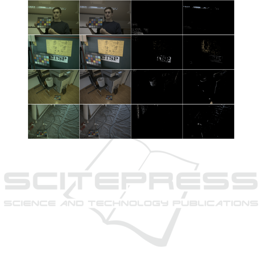
Figure 1: Detection of gray pixels. From left to right: input image, color-corrected image using ground-truth, pixels chosen

by the proposed method in Section 4.3, and pixels chosen by (Yang et al., 2015). Macbeth Color Checker are masked out due

to both methods ﬁnd gray pixels on gray regions.

led mean-shifted gray pixel, or MSGP, is a process

that detects pixels that are assumed to be gray under

neutral illumination. Why gray pixels? Gray or ne-

arly gray pixels are wide spread in indoor and out-

door images (Yang et al., 2015). In the process of

manufacturing camera, each camera is calibrated to

maintain: gray pixels will be rendered gray in linear

image (not raw response) under standard neutral illu-

mination. Gray pixel examples are shown in the third

column in Fig. 1.

Considering that gray pixels are informative w.r.t.

casting illumination, it is possible to transform the

scene illumination estimation task into gray pixel de-

tection. This paper proposes an accurate method for

the detection of gray pixels by combining a novel

grayness measure with Mean-shift clustering in color

space.

Experimental results in camera-agnostic color

constancy show that the proposed algorithm outper-

forms both statistical and learning-based methods of

the state-of-the-art. Even in the non camera-agnostic

scenario, i.e. using k-fold cross validation in the same

datasets, the proposed method outperforms other sta-

tistical methods and shows a competitive performance

when compared to learning-based methods.

2 PREVIOUS RELATED WORK

Assuming a photometric linear image I captured

using a digital camera, with pixels below black le-

vel and above saturation level corrected, the simpli-

ﬁed imaging formation under one global illumination

source can be expressed as (Gijsenij et al., 2011):

(x,y) =

L(λ)S

(λ)R(x,y,λ)dλ, i ∈{R,G,B}, (1)

where I

(x,y) is the measured image color value at

spatial location (x,y), L(λ) the wavelength distribu-

tion of the global light source, S

(λ) the spectral re-

sponse of the color sensor, R(x,y,λ) the surface re-

ﬂectance and λ the wavelength.

Under the narrow-band assumption (Von Kries

coefﬁcient law (von Kries, 1970)), Eq. 1 can be furt-

her simpliﬁed as (same as (Barron, 2015)):

I = W L, (2)

which shows that the whole captured image I is

the element-wise Hadamard product of the white-

balanced image W and the illumination L.

The goal of all color constancy methods, both

learning-based and statistical methods, is to estimate

L, so as to recover W , given I.

Learning-based Methods (Chakrabarti et al., 2012;

Gijsenij et al., 2010; Gehler et al., 2008; Gijsenij

Revisiting Gray Pixel for Statistical Illumination Estimation

and Gevers, 2011; Joze and Drew, 2014; Qian et al.,

2016; Qian et al., 2017) aim at building a model that

relates the captured image I and the sought illumi-

nation L from extensive training data. Among the

best-performing state-of-the-art approaches, the CCC

method discriminatively learns convolutional ﬁlters

in a 2D log-chroma space (Barron, 2015). This fra-

mework was subsequently accelerated using the Fast

Fourier Transform on a chroma torus (Barron and

Tsai, 2017). Chakrabarti et al. (Chakrabarti, 2015)

leverage the normalized luminance for illumination

prediction by learning a conditional chromaticity dis-

tribution. DS-Net (Shi et al., 2016) and FC

Net (Hu

et al., 2017) are two representative methods using

deep learning. The former network chooses an es-

timate from multiple illumination guesses using a

two-branch CNN architecture, while the later addres-

ses local estimation ambiguities of patches using a

segmentation-like framework. Learning-based met-

hods achieve great success in predicting pre-recorded

“ground-truth” illumination color to a fairly high

accurate level, but heavily depending on the same ca-

meras being used in both training and testing ima-

ges (see Sections 3 and 5.2). The Corrected-Moment

method (Finlayson, 2013) can also be considered as a

learning-based method as it needs to train a corrected

matrix for each dataset.

Statistical Methods estimate illumination by making

some assumptions about the local or global regula-

rity of the illumination and reﬂectance of the input

image. The simplest such method is Gray World (Bu-

chsbaum, 1980), that assumes that the global average

of reﬂectance is achromatic. The generalization of

this assumption by restricting it to local patches and

higher-order gradients has led to some classical and

recent statistics-based methods, such as White Patch

(Brainard and Wandell, 1986), General Gray World

(Barnard et al., 2002), Gray Edge (Van De Weijer

et al., 2007), Shades-of-Gray (Finlayson and Trezzi,

2004) and LSRS (Gao et al., 2014), among others

(Cheng et al., 2014). The closest works to ours are

Xiong et al. (Xiong et al., 2007) and Gray Pixel (Yang

et al., 2015). Xiong et al. (Xiong et al., 2007) ﬁnds

gray surfaces based on a special LIS space, but this

method is camera-dependent. The Gray Pixel method

will be discussed in Section 4.

Physics-based and other Methods (Tominaga, 1996;

Finlayson and Schaefer, 2001a; Finlayson and Schae-

fer, 2001b) estimate illumination from the understan-

ding of the physical process of image formation (e.g.

the Dichromatic Model), thus being able to model

highlights and inter-reﬂections. Most physics-based

methods estimate illumination based on intersection

of multiple dichromatic lines, making them work well

on toy images and images with only a few surfaces

but not very reliable on natural images (Finlayson and

Schaefer, 2001b). The latest physics-based method is

(Woo et al., 2018), which relies on the longest dichro-

matic line segment assuming Phong reﬂection model

holds and an ambient light exists. Although our met-

hod is based on the Dichromatic Model, we classify

our approach as statistical since the core of the met-

hod is ﬁnding gray pixels based on some observed

image statistics. We refer readers to (Gijsenij et al.,

2011) for more details about physics-based methods.

The contribution of this paper is three-fold:

• We experimentally demonstrate that, in the

camera-agnostic color constancy setting, state-of-

the-art learning-based methods are outperformed

by statistical methods

• We point out the hidden elongated pixel prior over

indoor and outdoor color constancy datasets.

• We present the Mean-shift-based Gray Pixel

method, robustly searching dominant illumina-

tion (mode) and achieving state-of-the-art perfor-

mance among competing training-free alternati-

ves. Code will be released upon publication.

3 CAMERA-AGNOSTIC COLOR

CONSTANCY

For a given camera, noted as C, Eq. 2 can be rewritten

as:

= W

, (3)

which indicates that both, the captured image I

, the

canonical image W

and the illumination L

that we

need to estimate, are dependent on the camera type C.

indicates that in canonical light, the images cap-

tured by different cameras of the same scene differ.

The color constancy problem in learning-based

methods can be stated as

= f (w,I

), where

the estimated illumination, and f (w,·) is the mapping

to be learned with parameters w. The mapping f (w,·)

can be embodied by various machine learning models

or an ensemble of them. If the learning process for a

particular dataset is guided by the distance (e.g. angu-

lar error) between

and L

, w will undoubtedly be

biased by the particular characteristics of the camera

C. In other words, the parameters of f (w,·) will be

learned to be “well-performing” on a speciﬁc dataset

that encompasses one or a few pre-selected cameras.

With the massive modeling capability of some ma-

chine learning models (e.g. regression trees and deep

learning), the camera sensibility function of a bag of

cameras can be modeled up to a high degree. In the li-

terature, the validation of color constancy methods is

VISAPP 2019 - 14th International Conference on Computer Vision Theory and Applications

customarily performed using k-fold cross-validation

on the same dataset. As a result, this validation pro-

cess favors learning-based methods and fails to assess

their performance for color correction in images from

an unknown camera (Gao et al., 2017).

In this work, we deﬁne camera-agnostic color

constancy as the problem of estimating the illumi-

nation L

of a color-biased image I

that has been

captured by a camera C of unknown properties. For

learning-based methods, this implies that the input

image I

has been captured by a camera not pre-

viously “seen” in the training process. Therefore,

a rigorous validation process of color constancy al-

gorithms should consider both, camera-agnostic and

known-camera scenarios. By leveraging publicly

available datasets, this can be achieved by training

in one dataset and testing in other without overlap-

ping cameras (see Section 5). In contrast to learning-

based methods, statistical methods have the advantage

of adjusting the model in a per-image basis thus ha-

ving the potential to implicitly deal with the camera-

agnostic problem.

4 MEAN-SHIFTED GRAY PIXEL

The proposed mean-shifted gray pixel algorithm, or

MSGP, is built on the assumption that achromatic

pixels in the corresponding canonical image can be

used to estimate the global illumination. Speciﬁcally,

achromatic pixels are visually gray in the color cor-

rected image. Yang et al. (Yang et al., 2015) clai-

med the mentioned assumption, and experimentally

demonstrated the presence of detectable gray pixels

in most natural scenes under white light. In this work,

we further extend the concept of the Gray Pixel met-

hod by means of an adaptive method for the detection

gray pixels that combines a new grayness function

and mean-shift clustering.

4.1 Original Gray Pixel (GP) Revisited

In this section, we revisited the original Gray Pixel

method (Yang et al., 2015), which is derived from a

limited diffuse reﬂection model. Applying a log trans-

formation to both sides of (2), we have:

log(I

(x,y)

) = log(W

(x,y)

) + log(L

) (4)

In a small enough local neighborhood, the illu-

mination L can be assumed as uniform under global

illumination constrains. As a result, the application

of a linear channel-wise local contrast operator C{·}

(Laplacian of Gaussian, which we will use for the re-

mainder of the paper) on (4) yields:

C{log(I

(x,y)

)} = C{log(W

(x,y)

)} (5)

Eq. (5) indicates a well-known observation: the cas-

ting illumination is irrelevant to the channel-wise lo-

cal contrast of a small local neighborhood (Geuse-

broek et al., 2001). It also means that regions with no

contrast are useless for obtaining illumination cues.

Following (Yang et al., 2015), with balanced R, G and

B responses, the following condition must be met by

gray pixels:

C{log(I

(x,y)

)} = C{log(I

(x,y)

)} = C{log(I

(x,y)

)} 6= 0.

(6)

In practice, (6) does not hold strictly. As a result,

it is necessary to propose a “grayness” measure in

order to detect nearly gray pixels. For the sake of

simplicity, let us deﬁne the local contrast of a log-

transformed image pixel located at (x,y) as ∆

(x,y) =

C{log(I

(x,y)

)} with i ∈ {R,G,B}. In (Yang et al.,

2015), the grayness measure of a pixel, G(x, y), is de-

ﬁned as:

G(x,y) =

∑

i∈{R,G,B}

(∆

(x,y) −

∆(x,y))

∆(x,y)

1/2

(7)

where

∆(x,y) is the average of channels R, G and B.

It is claimed that the smaller G(x, y) is, the more

gray a pixel is under white light. Then some post-

processing steps are applied to weaken dark pixels

(luminance as dominator) and isolated pixels (local

averaging), for which we refer readers to the original

GP (Yang et al., 2015).

A major drawback of Eq. 7 is that the grayness

estimate depends on the luminance of the pixels. Spe-

ciﬁcally, the effect of

∆ results in gray pixels having

different grayness values due to differences in lumi-

nance. Alternatively, we propose that grayness should

only depend on chromaticity. Therefore, in the next

section, we will introduce a new grayness function to

replace Eq. 7.

4.2 Grayness Function

We propose an ideal grayness function G(·) ∈ [0, 1]

where 0 denotes pure gray of a pixel color. Without

speciﬁcation, the grayness function works in RGB

space as it is closest to the image formation process

and main choice of in line of research (Yang et al.,

2015; Barron and Tsai, 2017). Our grayness function

should comply with the following properties:

Revisiting Gray Pixel for Statistical Illumination Estimation

Property

G(·) is invariant to the luminance

(sum of RGB values).

Property

G(·) outputs monotonically decre-

asing value for increasing visual

grayness, e.g. from red to white.

Property

Pure gray pixels (on the black-to-

white line) should be have value 0.

In addition the three above-mentioned properties,

it is also desirable that the output space of the gray-

ness function be normalized (so that no subsequent

normalization is required), as well as having a physi-

cal meaning so that it can be used for other computer

vision tasks. Alternatively to the grayness measure

proposed in (Yang et al., 2015), we propose a new

grayness measure based on the angular error function

that complies with all these properties:

G(x,y) = cos

−1



h∆(x,y), gi

k∆(x,y)kkgk



, (8)

where ∆(x,y) = [∆

,∆

]

is the RGB vector in

location (x,y), g is the gray light reference vector

]

, and k·k

refers to the n norm.

Our motivation behind Eq. 8 is that, even in the

color-biased scenario, it is possible to assume that all

gray colors captured by the same camera will have

balanced R, G, B components, regardless of their lu-

minance level. As a result, it is possible to assess their

grayness level by measuring the angular error with re-

spect to a reference gray value. Notice that, in ge-

neral, the gray reference vector g can have spatially-

varying values in order to adjust for changes in the il-

lumination of the scene. In this work, however, we as-

sume that the global illumination source remains con-

stant in the scene and adopt the canonical gray value

as reference: g = [1,1,1]

. In this case, Eq. 8 can be

further simpliﬁed as:

G(x,y) = cos

−1



√

k∆(x,y)k



, (9)

Eq. 9 measures how gray a pixel is, using the an-

gular distance from the local contrast vector to the

gray light g, thus meeting Properties 1 and 2. When

the point (x,y) is completely gray, G(x,y) is 0 and in-

creases monotonically with decreasing level of gray-

ness, thus meeting Property 3. In addition, the out-

put ranges from 0

◦

to cos

−1

(

√

) for each image, thus

being normalized.

Empirical Evidence – The next question is whether

this new grayness function brings different ordering

of pixels according to their grayness levels. To ans-

wer this, we replace Eq. 7 with Eq. 8 in the original

GP algorithm and estimate illumination in two main-

stream color constancy benchmarks where GP is eva-

luated. Table 1 shows the performance improvement

by a large margin (0.6

◦

reduction in median error for

SFU Color Checker) when we use the proposed gray-

ness measure Eq. 8. Results on the SFU Indoor data-

set do not differ much, arguably because the dataset is

collected in a laboratory environment with a restricted

set-up (many image feel artiﬁcial and examples are

shown in Fig 2). The proposed method is based on

the assumption of natural image statistics and works

for more general cases. For the results shown in Ta-

ble 1, the top 0.1% pixels with G values are chosen as

gray pixels, as recommended by (Yang et al., 2015).

The local contrast operator C{·} is the Laplacian of

Gaussian.

Table 1: Angular error of the Gray Pixel (Yang et al., 2015)

algorithm with different grayness functions: original gray-

ness function (GP) and proposed grayness function in Eq. 9

(GP

∗

SFU Color Checker SFU Indoor

Mean Med Trimean Mean Med Trimean

GP 4.6 3.1 – 5.3 2.3 –

∗

4.1 2.5 2.8 5.3 2.2 2.7

Figure 2: Examples of SFU Indoor dataset.

Here we mathematically analyze the connection

between the grayness function in Eq. 7 and the pro-

posed grayness measure in Eq. 9. To avoid readers’

confusion, we term the original grayness measure in

Eq. 7 as G

(x,y) and the proposed grayness function

of Eq. 8 as G

(x,y). In the sequel, we demonstrate

that G

and G

are related by:

(x,y) = γ(x,y)G

(x,y), (10)

where γ(x,y) is a luminance-dependent term.

In order to demonstrate the relationship in Eq. 10,

we approximate G

as follows

≈

1 −

√

k∆k

(11)

It can be readily shown that Eq. 11 is an approxi-

mation of the same order of Eq. 9 in the interval [0,1].

With this approximation, G

and G

can be rewritten

as:

3βG

= α

−3β

(12)

= 1 −

√

3β

(13)

For the sake of simplicity we will drop the pixel coor-

dinates (x,y) in the remaining of this section

VISAPP 2019 - 14th International Conference on Computer Vision Theory and Applications

where α = k∆k

and β =

k∆k

Putting a multiplier α(α +

√

3β) to both sides of

Eq. 13 yields:

α(α +

√

3β)G

= α

−3β

(14)

Finally, combing Eq. 12 and 14 we obtain the

sought relationship:

= γG

, (15)

where γ

equals to α(α +

√

3β)/3υ.

From Eq. 15 it is clear that the original gray-

ness function G

(x,y) contains not only the real gray-

ness – cosine distance G

(x,y) from the gray light –

but also introduces a non-linear luminance-dependent

term γ(x,y), which adds noise to the grayness esti-

mate. As a result, two points with same values of

(x,y) but different luminance values will yield dif-

ferent values of G

(x,y). In contrast, the proposed

grayness function G

(x,y) is more robust to changes

in luminance.

After some post-processing steps (e.g. local aver-

aging and normalization by image intensity), a small

percentage of pixels (N%) with the highest grayness

values (lowest G) are chosen and averaged to be the

illumination estimate. However, as it will be shown

in the next section, the chosen gray pixels may still

contain a number of colorful pixels. As a result, we

will apply Mean Shift clustering in 3D RGB space in

order to remove spurious color pixels. In the experi-

ments in the remaining of this paper, we will use the

new grayness function unless indicated otherwise.

4.3 Mean Shift Puriﬁcation

Let S be the set of preselected N% pixels according

to their grayness levels. Ideally, S should only con-

tain pure-gray pixels. However, in fact S may contain

a number of colorful pixels that need to be removed

before estimating the global illumination of the scene.

In order to remove color pixels from S, we note

that, for a color-biased image I, all the pure-gray

pixels should be contained in the illumination di-

rection [L

]. This is equivalent to having all

the pixels aligned towards the gray-light vector g =

[1,1, 1]

in the canonical image. For illustration pur-

poses, Fig. 3j shows all the pixels of the canonical

image of Fig. 3g in RGB space and Fig. 3k shows the

corresponding set S of pre-selected gray-pixels. From

Fig. 3k, it is clear that S contains both color and gray

pixels. As predicted by our assumption, most true-

gray pixels are aligned towards one single direction.

In particular, the main direction of the densest pixel

cloud indicates the illumination of the scene.

In this paper, we use mean shift (MS) clustering

(Fukunaga and Hostetler, 1975; Comaniciu and Meer,

2002) with a hybrid distance to seek for the dark-

to-bright elongated cluster which contains the most

pixels in S. MS is a non-parametric space analysis

algorithm, treating the feature space as a probability

density function and seeking for the modes. In this

work, the density of each pixel p ∈S in RGB space is

calculated as a function of the bandwidth h:

f (p) =

∑

i=1

K(p, p

;h), (16)

where n the number of pixels in S, and the kernel den-

sity function K(·) is deﬁned as:

K(p, p

;h) =

(

1, if D(p, p

) ≤ h

0, otherwise

(17)

with I(p) = [I

] being the vector with RGB va-

lues of pixel p, D(p, p

) is the deﬁned hybrid distance

computed as the product of the euclidean and angular

distances kI(p)−I(p

·∠{I(p),I(p

)}, and ∠{·}is

the angle between two vectors.

Finally, the centroid corresponding to the mode

with highest density is used for the computation of

the illumination estimate:

L = argmax

p∈S

f (p). (18)

The effect of mean shift clustering on the detection of

gray pixels is illustrated in Fig. 3. Comparing Figs. 3h

and 3i, it is clear how the mean-shift clustering, sim-

ply and effectively, allows for the detection and re-

moval of color pixels in the initial set S. It is worthy

to mention that, in some cases, there is almost no co-

lored pixels in S. Fortunately, the performance will

not suffer from clustering, as MS gracefully genera-

tes only one cluster which gives us a reliable estimate.

As a result, there is no need to condition when to ap-

ply clustering.

The mean-shifted gray pixel algorithm (MSGP) is

summarized in Algorithm 1. The proposed method

depends only in two parameters: the percentage of

pixels chosen from their grayness values, N%, and

the clustering bandwidth h of Eq. 16. The selection

of these parameters and their effect on the perfor-

mance of the proposed MSGP algorithm are presented

in section 5.3.

5 EXPERIMENTS

Experiments were conducted in two widely known,

publicly available datasets collected for the purpose

of evaluation of color constancy methods:

Revisiting Gray Pixel for Statistical Illumination Estimation

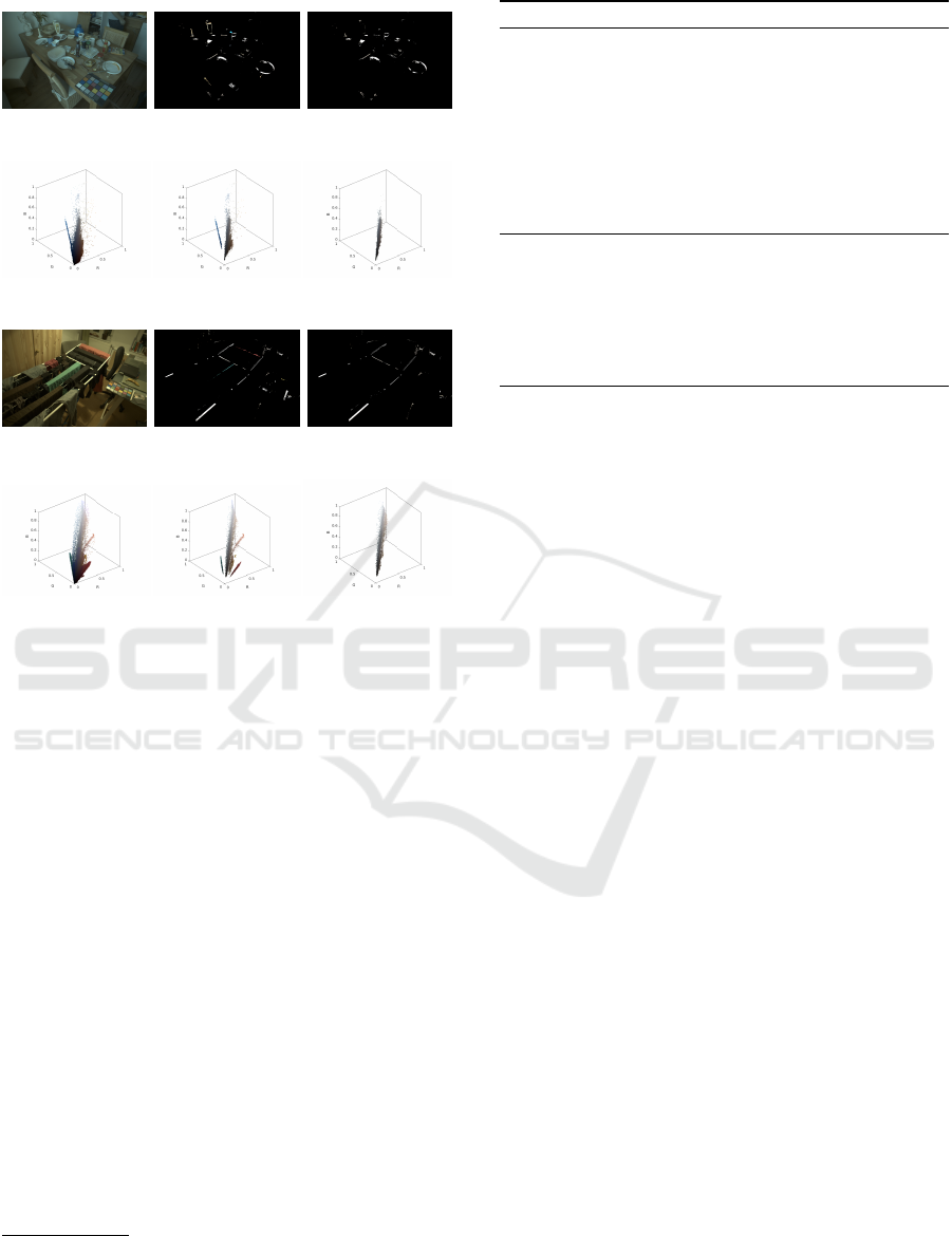
(a) (b) (c)

(d) (e) (f)

(g) (h) (i)

(j) (k) (l)

Figure 3: Detection of gray pixels. After correction using

ground-truth illumination, ideal gray pixel should looks pu-

rely gray. (a,g) Input image, (b,h) Initial gray pixels de-

tected. (c,i) Puriﬁed gray pixels after the Mean Shift step.

(d-f, j-l) color histograms of (a-c). Comparing (e) with (f),

(j) with (l), it is clear that Mean Shift helps to discard color

pixels in (e) that are not aligned with the main illumination

vector. For visualization purposes, the luminance of (b,c) is

multiplied by a constant 4.

• Gehler-Shi Dataset (Shi and Funt, 2010): 568

high dynamic linear images, 2 cameras

• NUS 8-Camera Dataset (Cheng et al., 2014):

1736 high dynamic linear images, 8 cameras

The parameters of the proposed MSGP algorithm

were selected as follows: the local contrast operator

used in Eq. 9 was the Laplacian of Gaussian with a

range of 5 pixels. The bandwidth for MS clustering

was set to h = 0.001. The percentage of pixels chosen

for the generation of S was set to N = 0.1%. These

parameters were selected based on preliminary expe-

riments (see Section 5.3) and remained ﬁxed for all

the experiments.

In order to allow for a rigorous comparison with

state-of-the-art methods, we have considered two sce-

cameras: Canon 1D, Canon 5D

cameras: Canon 1DS Mark3, Canon 600D, Fujiﬁlm

X-M1, Nikon D5200, Olympus E-PL6, Panasonic Lumix

DMC-GX1, Samsung NX2000, Sony SLT-A57

Algorithm 1: Mean-Shifted Gray Pixel.

Inputs:

I  Color-biased image

Parameters:

N  Percentage of pixels

h  Bandwidth for MS clustering

Output:

L  Estimated illumination.

Steps:

1. Compute local contrast ∆(x,y)

2. Compute grayness measure G

(x,y).  Eq. 8

3. Generate S with the top-N% gray pixels.

4. MS clustering on S with bandwidth h.  Eq. 16

5. Select

L as the strongest mode of

f .  Eq. 18

narios. The camera-agnostic setting and the camera-

known setting. In the agnostic-camera setting,

learning-based algorithms are trained in one dataset

(e.g., Gehler-Shi) and tested on the other. This al-

lows for testing the performance of the algorithm in

cameras not previously “seen” in the training process.

The camera-known setting corresponds to the typi-

cal 3-fold cross validation used in the literature, in

which learning-based methods are trained and valida-

ted in the same dataset. Visual comparison is given in

Fig. 1, where the proposed method detects gray pixels

more accurately. Numerical statistics are summarized

in Table 2 and discussed in Sections 5.2 and 5.1.

5.1 Camera-known Setting

Camera-known setting (also termed as single-dataset

setting) is the most common setting in related works,

allowing extensive pre-training using a k-fold valida-

tion for learning-based methods. The results for this

setting are summarized in table 2b. Among all the

compared methods, FFCC yields the best overall per-

formance in both datasets. It is important to remark

that, cross validation makes no difference in the per-

formance of statistical methods. Therefore, in order

to avoid repetition, the performance of competing sta-

tistical methods is not shown in this table (see next

section). Remarkably, it is clear that, even in the

known-camera setting, the proposed algorithm out-

performs several learning-based methods (from Ga-

mut (Gijsenij et al., 2010) to the Exemplar-based met-

hod (Joze and Drew, 2014)) without extensive training

and parameter tuning.

5.2 Camera-agnostic Setting

In order to allow for a fair comparison in the camera-

agnostic scenario, learning-based methods should be

VISAPP 2019 - 14th International Conference on Computer Vision Theory and Applications

Table 2: Comparison of color constancy methods. All values correspond to angular error in degrees. For (a,b) we retrieve the

results of the related works in the following order: 1) the cited paper, 2) Table [1] and Table [2] from Barron et al. (Barron

and Tsai, 2017; Barron, 2015) considered to be up-to-date and comprehensive, 3) the color constancy benchmarking website

(Gijsenij, 1999). We left dash on unreported results. In (b) results of learning-based methods worse than ours are marked in

gray. The training time and testing time are reported in seconds, averagely per image, if reported in the original paper.

(a) Camera-agnostic setting

Training set NUS 8-Camera Gehler-Shi Average

Testing set Gehler-Shi NUS 8-Camera runtime (s)

Mean Median Trimean Best 25% Worst 25% Mean Median Trimean Best 25% Worst 25% Train Test

Learning-based Methods (agnostic-camera setting), Our rerun

Bayesian 4.75 3.11 3.50 1.04 11.28 3.65 3.08 3.16 1.03 7.33 764 97

Chakrabarti et al. 2015 Empirical 3.49 2.87 2.95 0.94 7.24 3.87 3.25 3.37 1.34 7.50 – 0.30

Chakrabarti et al. 2015 End2End 3.52 2.71 2.80 0.86 7.72 3.89 3.10 3.26 1.17 7.95 – 0.30

Cheng et al. 2015 5.52 4.52 4.79 1.96 12.10 4.86 4.40 4.43 1.72 8.87 245 0.25

FFCC 3.91 3.15 3.34 1.22 7.94 3.19 2.33 2.52 0.84 7.01 98 0.029

Physics-based Methods

IIC 13.62 13.56 13.45 9.46 17.98 – – – – – – –

Woo et al. 2018 4.30 2.86 3.31 0.71 10.14 – – – – – – –

Biological Methods

Double-Opponency 4.00 2.60 – – – – – – – – – –

ASM 2017 3.80 2.40 2.70 – – – – – – – – –

Statistical Methods

White Patch 7.55 5.68 6.35 1.45 16.12 9.91 7.44 8.78 1.44 21.27 – 0.16

Grey World 6.36 6.28 6.28 2.33 10.58 4.59 3.46 3.81 1.16 9.85 – 0.15

General GW 4.66 3.48 3.81 1.00 10.09 3.20 2.56 2.68 0.85 6.68 – 0.91

2st-order grey-Edge 5.13 4.44 4.62 2.11 9.26 3.36 2.70 2.80 0.89 7.14 – 1.30

1st-order grey-Edge 5.33 4.52 4.73 1.86 10.43 3.35 2.58 2.76 0.79 7.18 – 1.10

Shades-of-grey 4.93 4.01 4.23 1.14 10.20 3.67 2.94 3.03 0.99 7.75 – 0.47

Grey Pixel (edge)

4.60 3.10 – – – 3.15 2.20 – – – – 0.88

LSRS 3.31 2.80 2.87 1.14 6.39 3.45 2.51 2.70 0.98 7.32 – 2.60

Cheng et al. 2014 3.52 2.14 2.47 0.50 8.74 2.93 2.33 2.42 0.78 6.13 – 0.24

Mean Shifted Gray Pixel 3.45 2.00 2.36 0.43 8.47 2.92 2.11 2.28 0.60 6.69 – 1.32

(b) Camera-known setting

Gehler-Shi NUS 8-camera

Mean Median Trimean Best 25% Worst 25% Mean Median Trimean Best 25% Worst 25%

Learning-based Methods (camera-known setting)

Edge-based Gamut 6.52 5.04 5.43 1.90 13.58 4.40 3.30 3.45 0.99 9.83

Pixel-based Gamut 4.20 2.33 2.91 0.50 10.72 5.27 4.26 4.45 1.28 11.16

Bayesian 4.82 3.46 3.88 1.26 10.49 3.50 2.36 2.57 0.78 8.02

Natural Image Statistics 4.19 3.13 3.45 1.00 9.22 3.45 2.88 2.95 0.83 7.18

Spatio-spectral (GenPrior) 3.59 2.96 3.10 0.95 7.61 3.06 2.58 2.74 0.87 6.17

Corrected-Moment

(19 Edge) 3.12 2.38 2.59 0.90 6.46 3.03 2.11 2.25 0.68 7.08

Corrected-Moment

(19 Color) 2.96 2.15 2.37 0.64 6.69 3.05 1.90 2.13 0.65 7.41

Exemplar-based

∗

2.89 2.27 2.42 0.82 5.97 – – – – –

Chakrabarti et al. 2015 2.56 1.67 1.89 0.52 6.07 – – – – –

Cheng et al. 2015 2.42 1.65 1.75 0.38 5.87 2.18 1.48 1.64 0.46 5.03

DS-Net (HypNet+SelNet) 1.90 1.12 1.33 0.31 4.84 2.24 1.46 1.68 0.48 6.08

CCC (dist+ext) 1.95 1.22 1.38 0.35 4.76 2.38 1.48 1.69 0.45 5.85

(AlexNet) 1.77 1.11 1.29 0.34 4.29 2.12 1.53 1.67 0.48 4.78

FFCC 1.78 0.96 1.14 0.29 4.62 1.99 1.31 1.43 0.35 4.75

Mean Shifted Gray Pixel 3.45 2.00 2.36 0.43 8.47 2.92 2.11 2.28 0.60 6.69

For Correct-Moment (Finlayson, 2013) we report reproduced and more detailed results by (Barron, 2015), which slightly differs with the original results:

mean: 3.5, median: 2.6 for 19 colors and mean: 2.8, median: 2.0 for 19 edges on Gehler-Shi Dataset.

We rerun Grey Pixel (edge) on NUS dataset.

∗

We mark Exemplar-based method with asterisk as it is trained and tested on a uncorrected-blacklevel dataset.

re-trained for evaluation in the same conditions as sta-

tistical methods. Several state-of-the-art CNN-based

methods are not publicly available. In this work,

we were able to re-run the Bayesian method (Gehler

et al., 2008), Chakrabarti et al.(Chakrabarti, 2015),

FFCC (Barron and Tsai, 2017), and the method by

Cheng et al. 2015 (Cheng et al., 2015), using the co-

des provided by the original authors. Note that this

list of methods includes FFCC, which showed the best

overall performance in the camera-known setting.

We train on one dataset and test on the other one.

Both datasets share no common cameras, thus meet-

ing our requirement of being “camera-agnostic”. For

the results reported in this section, we use the best or

ﬁnal setting for each method: Bayes (GT) for Baye-

sian; Empirical and End-to-End training for Chakra-

barti et al. (Chakrabarti, 2015); 30 regression trees

for Cheng et al.; full image resolution and 2 chan-

Revisiting Gray Pixel for Statistical Illumination Estimation

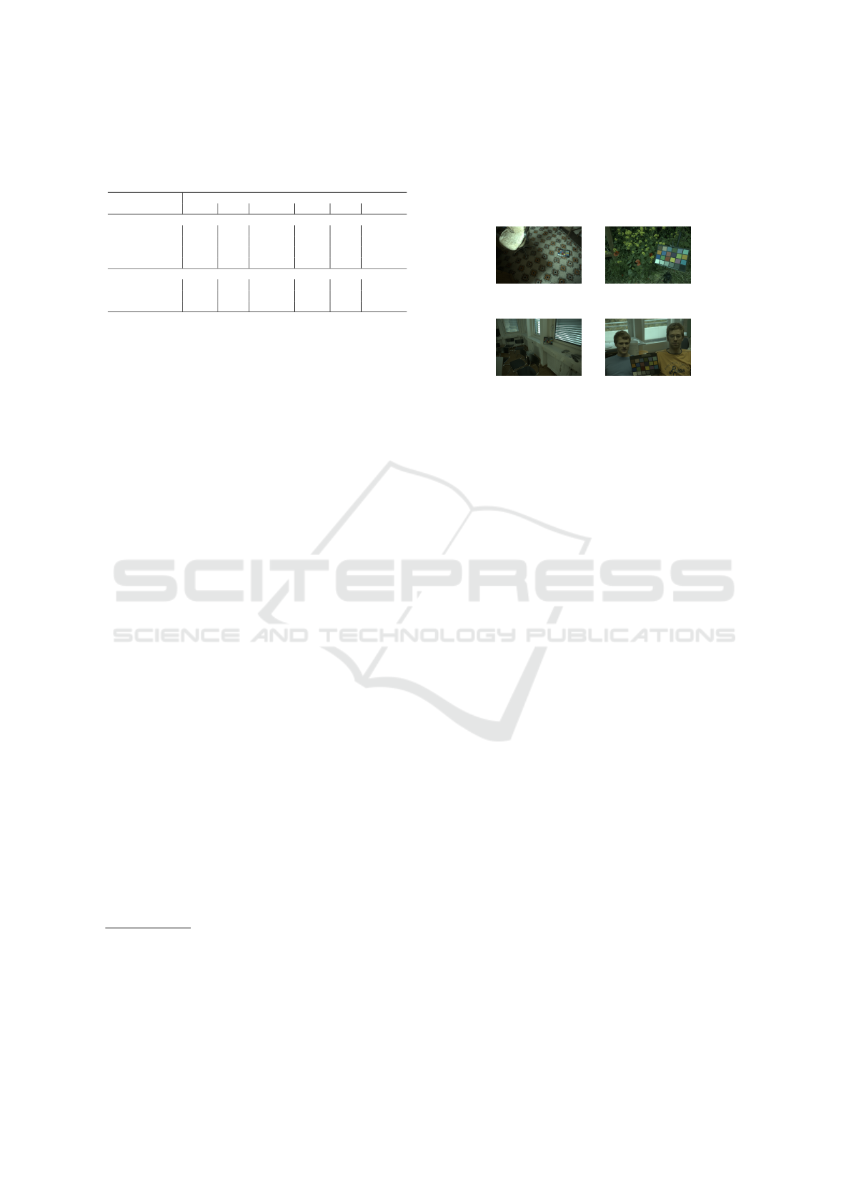
Table 3: Comparison between Mean Shift Clustering vs.

K-means Clustering in our task. “angle” refers to using an-

gular distance only in Mean Shift instead of the proposed

hybrid distance.

SFU Color Checker NUS 8-Camera

Mean Med Trimean Mean Med Trimean

Mean Shift

h=1e−3 (angle) 3.62 2.08 2.42 3.00 2.10 2.26

h=1e−4 3.51 2.04 2.38 3.32 2.13 2.39

h=1e−3 3.45 2.00 2.36 2.92 2.11 2.28

h=1e−2 3.48 2.11 2.44 3.00 2.19 2.39

Kmeans

K=2 3.75 2.18 2.54 3.00 2.10 2.28

K=5 4.44 2.46 2.73 3.32 2.13 2.37

K=9 4.50 2.51 2.80 3.37 2.19 2.39

nels for FFCC

. Obtained results are summarized in

Table 2a.

Obtained results are summarized in Table 2a.

From this table, it is clear that the proposed MSGP

algorithm outperforms both learning-based and statis-

tical methods. Except FFCC, selected learning-based

methods perform relatively worse in camera-agnostic

setting, as compared to statistical methods. Due to

their nature, it is not surprising that learning-based

methods degrade in their performance in the camera-

agnostic scenario. However, the fact that learning-

based methods are outperformed by statistical met-

hods is an interesting ﬁnding. On one side, if we

use learning-based methods trained for a given da-

taset or ”a bag of camera models”, we may fail in

the camera-agnostic setting. In contrast, in the both

camera-agnostic/known setting, the proposed statisti-

cal method provides stable performance.

5.3 Algorithm Parameters

The Role of Bandwidth h. The bandwidth h deter-

mines the domain size where Mean Shift computes

the pixel divergence. Here we evaluate variants of the

proposed method by changing h to be 1e−4, 1e−3

and 1e−2. Table 3 shows that the bandwidth 1e−3

gives a good trade-off between mean and median er-

ror on two datasets. For reference purposes, Table 3

also includes performance results obtained when the

distance function in Eq. 17 uses only angular infor-

mation in D(·).

Clustering Algorithm. We compare two clustering

methods, Mean Shift and K-means

. Here we eva-

luate variants of K-means by changing the number of

clusters K to 2, 5 and 9. Table 3 shows that, in general,

MS gives better results. This can be attributed to the

Scripts for re-running these methods will also be pu-

blic.

We use clustering to ﬁnd the mode i.e. the dominating

illumination color, while we don’t need all all clustered in-

dexes. We note that other clustering methods (e.g. spectral

clustering) may work well. We selected Mean Shift due to

its fast computation and robustness to the outliers.

fact that Mean Shift is more robust to outliers than K-

means. Among all K-means invariants, the 2-cluster

setting performs best. This suggests that S usually

contains 1 −2 elongated clusters.

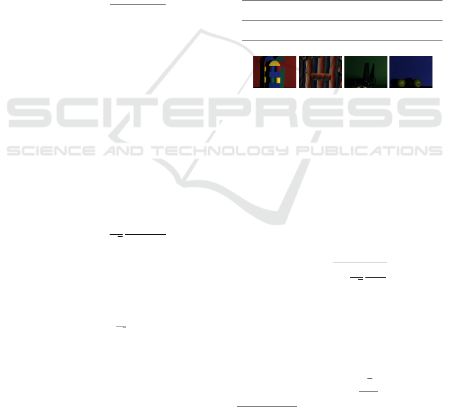
(a) 15.18

◦

(b) 26.13

◦

(d) 15.77

◦

Figure 4: Example failure cases with their angular errors.

(a,b) are examples with no detectable gray pixels (note that

the ground truth color chart is masked in evaluation). (c,d)

are examples with mixed illumination: indoor illumination

and outdoor illumination.

6 LIMITATIONS AND

CONCLUSIONS

Our method relies on gray pixels and their statis-

tics for one global illumination estimation. There-

fore, in some extreme cases, when there are no de-

tectable gray pixels or there are gray pixels repre-

senting two not-same-color illuminations, our method

fails. In Figure 4, two no-gray-pixel examples and

two double-illumination examples are shown. Cheng

et al. (Cheng et al., 2016) claimed that in SFU Co-

lor Checker Dataset (Shi and Funt, 2010), there are

66 two-illumination images (image list released). It is

worthy to mention that the images where we fail over-

lap largely with this two-illumination list. As mixed-

illumination problem is a different task and out of the

scope of this paper, we refer readers to (Cheng et al.,

2016) for details.

In this paper, we presented a statistical method for

tackling the problem of color constancy. The propo-

sed method relies on gray pixel detection and mean

shift clustering in order to estimate the illumination

of the scene based on the statistical properties of the

gray pixels of the input image. In the camera-agnostic

scenario, in which color constancy is to be applied to

images captured with unknown cameras, the proposed

method outperforms both learning-based and statisti-

cal state-of-the-arts.

The proposed method is easy to implement,

training-free, and depends only on two parameters,

namely the percentage of gray pixels N% and the

VISAPP 2019 - 14th International Conference on Computer Vision Theory and Applications

Mean Shift bandwidth h. With our method, proces-

sing a 2000 ×1500 linear RGB image takes about

1.32 seconds with unoptimized MATLAB code run-

ning in a CPU Intel i7 2.5 GHz. The method can be

adapted to other color spaces (e.g. Lab) without any

performance drop.

REFERENCES

Barnard, K., Cardei, V., and Funt, B. (2002). A comparison

of computational color constancy algorithms. i: Met-

hodology and experiments with synthesized data. TIP,

11(9):972–984.

Barron, J. T. (2015). Convolutional color constancy. In

ICCV.

Barron, J. T. and Tsai, Y.-T. (2017). Fast fourier color con-

stancy. In CVPR.

Brainard, D. H. and Wandell, B. A. (1986). Analysis of the

retinex theory of color vision. JOSA A, 3(10):1651–

1661.

Buchsbaum, G. (1980). A spatial processor model for object

colour perception. Journal of the Franklin Institute,

310(1):1–26.

Chakrabarti, A. (2015). Color constancy by learning to pre-

dict chromaticity from luminance. In NIPS.

Chakrabarti, A., Hirakawa, K., and Zickler, T. (2012). Co-

lor constancy with spatio-spectral statistics. TPAMI,

34(8):1509–1519.

Cheng, D., Kamel, A., Price, B., Cohen, S., and Brown,

M. S. (2016). Two illuminant estimation and user cor-

rection preference. In CVPR.

Cheng, D., Prasad, D. K., and Brown, M. S. (2014). Illu-

minant estimation for color constancy: why spatial-

domain methods work and the role of the color distri-

bution. JOSA A, 31(5):1049–1058.

Cheng, D., Price, B., Cohen, S., and Brown, M. S. (2015).

Effective learning-based illuminant estimation using

simple features. In CVPR.

Comaniciu, D. and Meer, P. (2002). Mean shift: A ro-

bust approach toward feature space analysis. TPAMI,

24(5):603–619.

Finlayson, G. D. (2013). Corrected-moment illuminant es-

timation. In ICCV, pages 1904–1911.

Finlayson, G. D. and Schaefer, G. (2001a). Convex and

non-convex illuminant constraints for dichromatic co-

lour constancy. In CVPR, volume 1, pages I–I. IEEE.

Finlayson, G. D. and Schaefer, G. (2001b). Solving for

colour constancy using a constrained dichromatic re-

ﬂection model. IJCV, 42(3):127–144.

Finlayson, G. D. and Trezzi, E. (2004). Shades of gray

and colour constancy. In Color Imaging Conference

(CIC).

Foster, D. H. (2011). Color constancy. Vision research,

51(7):674–700.

Fukunaga and Hostetler (1975). The estimation of the gra-

dient of a density function, with applications in pattern

recognition. IEEE Transactions on Information The-

ory, 21:32–40.

Gao, S., Han, W., Yang, K., Li, C., and Li, Y. (2014). Fef-

ﬁcient color constancy with local surface reﬂectance

statistics. In ECCV.

Gao, S.-B., Zhang, M., Li, C.-Y., and Li, Y.-J. (2017). Im-

proving color constancy by discounting the variation

of camera spectral sensitivity. JOSA A, 34(8):1448–

1462.

Gehler, P. V., Rother, C., Blake, A., Minka, T., and Sharp, T.

(2008). Bayesian color constancy revisited. In CVPR.

Geusebroek, J.-M., Van den Boomgaard, R., Smeulders,

A. W. M., and Geerts, H. (2001). Color invariance.

TPAMI, 23(12):1338–1350.

Gijsenij, A. (1999). Color constancy research website:

http://colorconstancy.com.

Gijsenij, A. and Gevers, T. (2011). Color constancy using

natural image statistics and scene semantics. TPAMI,

33(4):687–698.

Gijsenij, A., Gevers, T., and Van De Weijer, J. (2010).

Generalized gamut mapping using image derivative

structures for color constancy. IJCV, 86(2-3):127–

139.

Gijsenij, A., Gevers, T., and Van De Weijer, J. (2011). Com-

putational color constancy: Survey and experiments.

TIP, 20(9):2475–2489.

Hu, Y., Wang, B., and Lin, S. (2017). Fully convolutional

color constancy with conﬁdence-weighted pooling. In

CVPR.

Joze, H. R. V. and Drew, M. S. (2014). Exemplar-based

color constancy and multiple illumination. TPAMI,

36(5):860–873.

Qian, Y., Chen, K., K

ainen, J., Nikkanen, J., and Ma-

tas, J. (2016). Deep structured-output regression lear-

ning for computational color constancy. In ICPR.

Qian, Y., Chen, K., K

ainen, J., Nikkanen, J., and Ma-

tas, J. (2017). Recurrent color constancy. In ICCV.

Shi, L. and Funt, B. (2010). Re-processed version of the

gehler color constancy dataset of 568 images. acces-

sed from http://www.cs.sfu.ca/ colour/data/.

Shi, W., Loy, C. C., and Tang, X. (2016). Deep specialized

network for illumination estimation. In ECCV.

Tominaga, S. (1996). Multichannel vision system for esti-

mating surface and illumination functions. JOSA A,

13(11):2163–2173.

Van De Weijer, J., Gevers, T., and Gijsenij, A. (2007). Edge-

based color constancy. TIP, 16(9):2207–2214.

von Kries, J. (1970). Inﬂuence of adaptation on the ef-

fects produced by luminous stimuli. Source of Color

Science, pages 109–119.

Woo, S.-M., Lee, S.-h., Yoo, J.-S., and Kim, J.-O. (2018).

Improving color constancy in an ambient light en-

vironment using the phong reﬂection model. TIP,

27(4):1862–1877.

Xiong, W., Funt, B., Shi, L., Kim, S.-S., Kang, B.-H., Lee,

S.-D., and Kim, C.-Y. (2007). Automatic white ba-

lancing via gray surface identiﬁcation. In Color and

Imaging Conference (CIC).

Yang, K.-F., Gao, S.-B., and Li, Y.-J. (2015). Efﬁcient

illuminant estimation for color constancy using grey

pixels. In CVPR.

Revisiting Gray Pixel for Statistical Illumination Estimation

APPENDIX

Detailed Settings of Learning-based

Methods

To evaluate the performance of learning-based met-

hod in camera-agnostic scenario, we re-run the Baye-

sian method (Gehler et al., 2008), Chakrabarti et al.

2015 (Chakrabarti, 2015), FFCC (Barron and Tsai,

2017), and the method by Cheng et al. 2015 (Cheng

et al., 2015), using the codes provided by the aut-

hors. FFCC shows the best overall performance in the

camera-known setting. Our experimental settings for

re-running the aforementioned algorithms are sum-

marized below:

Bayesian method

(Gehler et al., 2008)

Among all variations of

Bayesian methods stated

in (Gehler et al., 2008), we

use Bayes (GT) but wit-

hout indoor/outdoor split,

to which Bayes (tanh) is

sensible. The ground truth

of training illuminations

(e.g. Gehler-Shi) is used as

point-set prior for testing

on the other dataset (e.g.

NUS 8-camera)

Chakrabarti et al.

2015 (Chakrabarti,

2015)

We use both variations gi-

ven by the author: the

empirical and the end-to-

end trained method. We

keeps all training hyperpa-

rameters same, e.g. epoch

number, momentum and

learning-rate for SGD.

FFCC (Barron and

Tsai, 2017)

For fair comparison, we

use Model (J) (FFCC

full,4 channels) in (Barron

and Tsai, 2017), which is

free of camera metadata

and semantic information

but still state-of-the-art.

Cheng et al. 2015

(Cheng et al., 2015)

Same as (Cheng et al.,

2015), we use four 2D fe-

atures with an ensemble of

regression trees (K=30).

VISAPP 2019 - 14th International Conference on Computer Vision Theory and Applications