SurfOpt: A New Surface Method for Optimizing the Classification of
Imbalanced Dataset
Andr
´
e Rodrigo da Silva, Leonardo M. Rodrigues and Luciana de Oliveira Rech
Department of Informatics and Statistics (INE), Federal University of Santa Catarina (UFSC)
Rua Delfino Conti, s/n, Trindade, Cx.P. 476, CEP: 88040-900, Florian
´
opolis, Brazil
Keywords:
Machine Learning, Skewed Classes, Imbalanced Datasets, Binary Classification.
Abstract:
Imbalanced classes constitute very complex machine learning classification problems, particularly if there are
not many examples for training, in which case most algorithms fail to learn discriminant characteristics, and
tend to completely ignore the minority class in favour of the model overall accuracy. Datasets with imbalanced
classes are common in several machine learning applications, such as sales forecasting and fraud detection.
Current strategies for dealing with imbalanced classes rely on manipulation of the datasets as a means of
improving classification performance. Instead of optimizing classification boundaries based on some measure
of distance to points, this work directly optimizes the decision surface, essentially turning a classification
problem into a regression problem. We demonstrate that our approach is competitive in comparison to other
classification algorithms for imbalanced classes, in addition to achieving different properties.
1 INTRODUCTION
In many scenarios of practical application of machine
learning, such as sales forecasting (Syam and Sharma,
2018), epidemic prevention (Guo et al., 2017), fraud
detection (Carneiro et al., 2017), and disease evolu-
tion (Zhao et al., 2017), the subpopulation (or class
of interest) may consist of a derisory portion of
the observed events, as in the analogy “needle in a
haystack”, but even harder than that. The events ob-
served as data points may be indistinguishable from
one another for prediction purposes. For example, the
next customer to close a deal with an online business
may have many, if not all, characteristics of a cus-
tomer who has not closed a deal in the past.
As it is not always feasible to sample all the rel-
evant characteristics of a population, the discriminat-
ing characteristics of a population are commonly ne-
glected. This causes the classifier’s performance to
fall due to the fact that the data points began to ap-
pear closer and show more similarity, with overlap-
ping class distributions, which makes decision bound-
aries subject to uncertainty. This work addresses typ-
ical problems in this type of scenario.
Although binary classification problems are not
hard classification problems alone, characteristics on
the data points and intricacies of the problem can add
further complexity. Typical examples of such char-
acteristics are classes being severely skewed, not lin-
early separable, the set of features being of both cate-
gorical and continuous variables, and the observations
being of sparse nature. Even algorithms that result
in complex non-linear classification models will tend
to stop classifying examples as being of the minority
class altogether under skewness to minimize classifi-
cation error.
The accuracy metric is the most popular measure
of a classifier’s performance since accuracy suffices
as a metric for classification with balanced classes.
For datasets with imbalanced classes, accuracy is mis-
leading – as it is biased to the majority class – and
insensitive to changes in the quality of classification
of the minority class. For example, sales prediction is
a scenario where accuracy limitations come into play.
In this case, it is essential to know how many times
buying customers (i.e. the minority class) were cor-
rectly predicted and to quantify to which fraction of
the total buying customers events it corresponds. A
model can be right every time it predicts a buying cus-
tomer, but if its predictions of non-buying customers
are not also perfect, it can still be misclassifying most
of the buying customers.
Cross-validation of binary classifiers results in
four primary metrics, true positives (TP), true nega-
tives (TN), false positives (FP), and false negatives
(FN). From these metrics, it becomes possible to com-
724
Rodrigo da Silva, A., Rodrigues, L. and Rech, L.
SurfOpt: A New Surface Method for Optimizing the Classification of Imbalanced Dataset.
DOI: 10.5220/0007407107240730
In Proceedings of the 11th International Conference on Agents and Artificial Intelligence (ICAART 2019), pages 724-730
ISBN: 978-989-758-350-6
Copyright
c
 2019 by SCITEPRESS – Science and Technology Publications, Lda. All rights reserved

pose more advanced metrics, such as specificity or
also called True Negative Rate (TNR), which mea-
sures the rate of negative examples being predicted
correctly versus the total negative cases. Another use-
ful metric is the Negative Predictive Value (NPV),
which is the ratio between the number of correctly
predicted negative cases and the total number of pre-
dicted negative cases. When dealing with skewed
data, the accuracy metric of a classifier tends to be
very stable and unable to represent changes of speci-
ficity or negative predictive value (assuming minority
class as negative). Recent years have been of growing
interest on better overall metrics to evaluate a clas-
sifier that can represent changes in the prediction of
the minority class, such as the F-measure (F1) (Lipton
et al., 2014) and the Matthews Correlation Coefficient
(MCC) (Boughorbel et al., 2017).
This paper presents an algorithm that handles clas-
sifications tasks with data imbalance and evaluates its
classification behaviour. The main contributions of
this work are the following:
• The novel SurfOpt algorithm, which is able to
handle properly data imbalance;
• A parameter-based strategy that allows to directly
optimize the classification surface;
• A three-metric diagnostic approach for perfor-
mance issues on classifiers;
The next sections of this paper are organised as
follows. Section 2 presents the related work. Sec-
tion 3 includes essential concepts for the development
of this work. Section 4 introduces the SurfOpt algo-
rithm, which is the main contribution of this work.
Section 5 presents an evaluation of the proposed al-
gorithm. Section 7 concludes the paper and presents
suggestions for future work.
2 RELATED WORK
This section presents the work related to this research,
including those considered essential in the areas of
machine learning classification, support vector ma-
chines, and boosting-and-bagging algorithms.
2.1 Machine Learning Classification
A classification task is a problem where a population
(e.g. flowers) needs to be discriminated in its dif-
ferent classes (e.g. iris setosa, versicolor, virginica),
whereas automated classification consists of learning
a function that maps input features (i.e. individual
characteristics) to outputs (i.e. class labels).
2.2 Support Vector Machines (SVM)
Linear separable classes can be easily classified by a
model generated by the SVM algorithm, which works
by finding an n −1 dimensional hyperplane that sepa-
rates classes in a n dimensional space, maximising the
margin between the hyperplane and each set of points.
This algorithm is convex, meaning that it always find
the optimal solution. Not linearly separable classes
can also be efficiently classified with SVM by using
a kernel. The kernel-trick projects points in a higher
dimensional space where they are linearly separable
(Boser et al., 1992; Hofmann, 2006). When used in
a two-dimensional space, SVM is equal to dividing
points with a straight line.
2.3 Boosting and Bagging
Adaboost and Adabag algorithms are ensemble meth-
ods that work by iteratively improving classification
results with weak classifiers. The ensemble model
of an Adaboost algorithm elects to which class every
observation belongs by using a weighted vote strat-
egy, where the weights of each classifier votes are
learned during training. Adabag uses a simple major-
ity vote strategy, and classifiers added to the ensem-
ble in every iteration are independent of the previous
classifiers, opposing Adaboost, which derives clas-
sifiers from previous iterations (Alfaro et al., 2013;
Schapire, 2013).
2.4 Oversampling and Undersampling
Recent work for imbalanced dataset classification
use non-algorithmic solutions, such as oversampling,
undersampling or a combination of both strategies
(Haixiang et al., 2017). Oversampling approaches
artificially increase the number of data-points of the
minority class. Undersampling techniques consist of
removing data-points of the majority class to balance
the dataset. These techniques manipulate the dataset
as a mean to improve the classifier performance.
2.5 Surface Optimization
Algorithms for classification generally optimize a
classification boundary based on some distance-to-
point metric (i.e. large margin classifiers). These
algorithms showed satisfactory convergence proper-
ties and great accuracy in many practical applications.
The weakness of this kind of algorithm lies in its sen-
sibility to outliers, and the fact they optimize for indi-
vidual points and not for the entire set, making classi-
fiers subject to bias found in data.
SurfOpt: A New Surface Method for Optimizing the Classification of Imbalanced Dataset
725

SurfOpt optimizes decision surface directly, being
able to learn trade-off regions for classification, and
being resilient to outliers as the influence of individual
data points diminishes as the number of data points
grow. We show that even maximum margin classifiers
with polynomial kernels such as SVM are unable to
capture trade-off regions on imbalanced data.
3 BACKGROUND
In this section, we will shortly review two concepts
that are important to the SurfOpt algorithm formula-
tion and evaluation.
3.1 Matthews Correlation Coefficient
Equation (1) presents the Matthews Correlation Coef-
ficient (MCC), which can be undefined if any of the
measures TP, TN, FP, TN are equal to zero. The ad-
dition of an infinitesimal positive constant to the de-
nominator of the formula solves that problem. The
MCC equation outputs in the interval [1, −1] if the
MCC of a classifier is 1, which is perfectly correct.
On the other hand, an MCC of −1 means a perfectly
incorrect classifier.
MCC =
T P× T N − F P × FN
p
(T P + F P) × (T P + FN) × (T N + FP) × (T N + FN)
(1)
3.2 Convex hull
The convex hull of a set of points is the smallest con-
vex set that contains the points (Barber et al., 1996).
The points on a convex hull define the vertices of a
polygon that contains the entire set. Some implemen-
tations of the convex hull run on linear expected time
(Devroye and Toussaint, 1981). In this work, we show
how to avoid finding convex hull of sets and distance-
to-point calculations by optimising a curve equation,
and a transformation of the data-points.
4 SurfOpt: OPTIMISING
CLASSIFICATION SURFACE
When classifying data-points of populations that
overlap one another, a non-smooth threshold for the
decision boundary such as a single straight line will
fail to capture the region of best classification trade-
off. To best capture the trade-off region, we envi-
sioned a weak classifier with a non-linear decision
boundary. Our classifier boundary is a curve, defined
by the function below:
f (a) = a
2
∗ exp(ω) (2)
The curve defined by Equation (2) is convenient
as it never assumes negative values. For large positive
values of ω, it approximates a vertical line and, for
small negative values of ω, it approximates a horizon-
tal line. From Equation (2), we learn the parameter
ω that define the width of the arc. To classify data-
points outside of the curve, it is necessary to do a ker-
nel transformation. Thus, concomitantly, we learn a
transformation to the points. The parameter θ defines
the angle of rotation to apply to every point P(a, b) in
relation to the origin point P(0, 0).
b = f (a) (3)
a
0
= a cos(θ) − b sin(θ) (4)
b
0
= a sin(θ) + b cos(θ) (5)
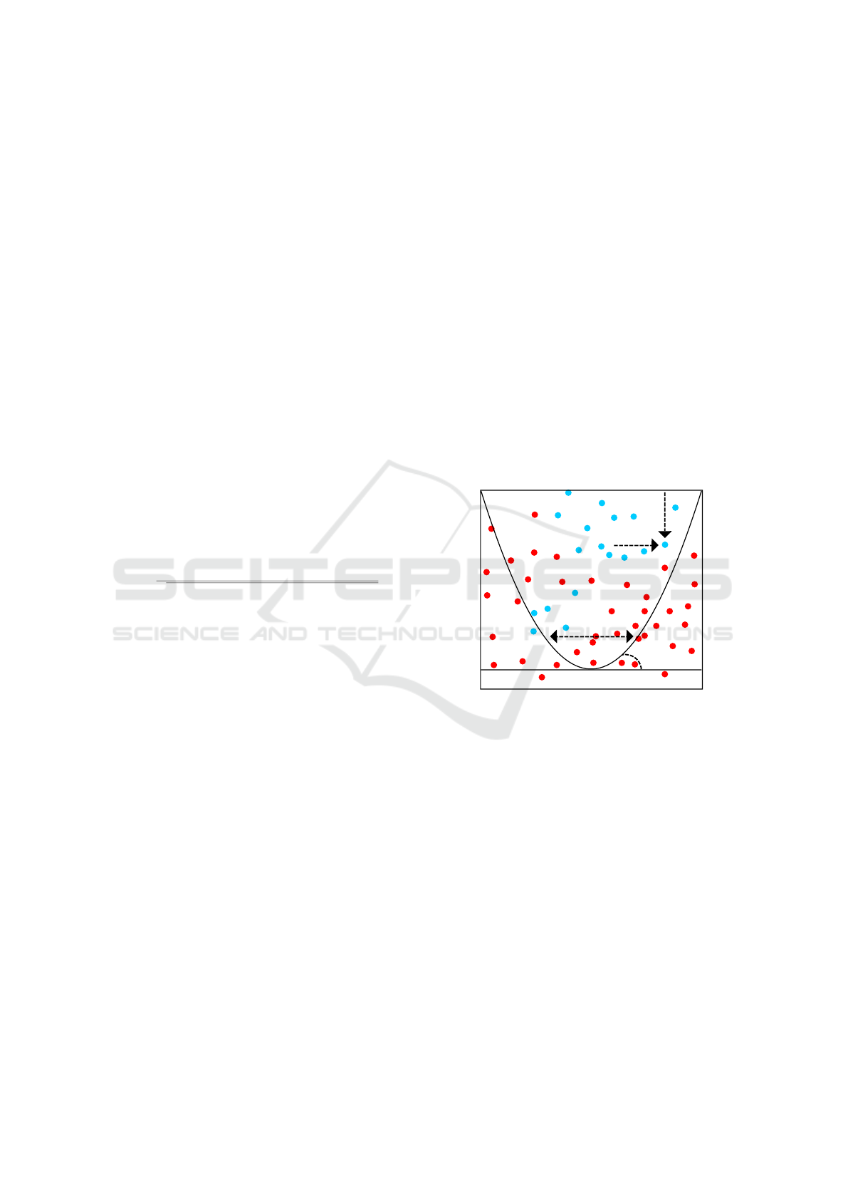
In addition to the rotation transformation, we add
the parameters c and d to shift every point a and b
coordinates in relation to the origin point P(0, 0), as
depicted in Figure 1.
ω
(0,0)
θ
c
d
Figure 1: Curve boundary and transformations to the points.
k
a
(a) = a cos(θ) − b sin(θ) + c (6)
k
a
(b) = a sin(θ) + b cos(θ) + d (7)
Equations (6) and (7) transform the x-axis and the
y-axis of the points on the plane, respectively. Once
a curve decision boundary is set and the points trans-
formed, we then use the Heaviside step function as
the decision function of our algorithm.
g(a) = k
b
(a) − f (a) (8)
H(a) =
(
0, if g(a) < 0
1, if g(a) ≥ 0
(9)
First, Equation 8 determines if a point is below or
above (i.e. inside) the curve after the transformation.
Then, if it is inside, Equation 9 labels the point as be-
ing of the minority class – denoted by 1 (one) – or the
majority class – denoted by 0 (zero).
ICAART 2019 - 11th International Conference on Agents and Artificial Intelligence
726

The area defined by the curve within the range
of the data-points is an ellipse-segment, every point
inside of it is predicted to belong to the minority
class. The algorithm evaluates the classifier perfor-
mance and yields a value x ∈ [0, 1] for classifier accu-
racy. In order to maximise x, we use the logistic loss,
which can be defined as follows:
Cost(x, y) =
(
−log(h
θ
(x)), if y=1
−log(1 − h
θ
(x)), if y=0
(10)
In Equation (10) h
θ
(x) denotes the hypothesis func-
tion with parameters θ with input x, our hypothesis
function are (6,7), we assume y to be always equal to
1 since it is the maximum value for the accuracy met-
ric (perfect classifier) that we want to achieve. With
Equation 10, we are able to calculate the gradient de-
scent and penalise the parameters of our hypothesis
function every iteration.
We calculate the gradient of the parameters with
the sigmoid function, i.e. f (x) =
1
1+e
−x
, to minimize
the error. We experimented different gradient descent
algorithms such as Adam(Kingma and Ba, 2015) and
Adagrad(Duchi et al., 2011), AMSgrad (Reddi et al.,
2018) showed the best results. The AMSgrad pro-
ceeds to update the transformations parameters, i.e.
Equations (6) and (7). Usually, the gradient descent
algorithm would repeat the optimization steps until
the max-number of iterations or the final performance
is reached. In our algorithm, we use a restart routine
whenever TNR and TPR metrics are below a thresh-
old, as a way to avoid over-fitting of the accuracy met-
ric. When the algorithm stops, we select the curve
which resulted in the best MCC on the training set.
4.1 SurfOpt: Algorithm
This section presents the logic used in SurfOpt ap-
proach. Algorithm 1 describes the procedures per-
formed for this optimising the classification surface.
Algorithm 1: SurfOpt.
S data points;
C
i
points on the curve;
E
i
current evaluation of the iteration i;
L labels of points;
c x-offset of the curve origin;
d y-offset of the curve origin;
θ rotation angle;
ω parameter, from Equation (2);
N true negative rate threshold;
P true positive rate threshold;
M maximum iterations for the gradient descent;
r resolution, number of points sampled in the curve;
α learning rate;
function SAMPLECURVEPOINTS(S, R, c, d, θ, ω)
Sample R points from a parabola within some range
beyond the data points, transformed to the parameters c,
d, θ, ω with Equations (6) and (7).
return C
end function
procedure RESTARTCURVEPOSITION(c,d,θ,b)
sets c (x-offset) as a random value within [1, −1]
times the sample standard deviation in x-axis;
sets d (y-offset) as a random value within [1, −1]
times the sample standard deviation in y-axis;
sets θ (rotation) with a random value within [2, 4]×π;
resets ω to its original value;
end procedure
function CLASSIFIEREVALUATION(S, C
i
)
Transforms data-points: every point inside the arc of
the curve defined by Equation (2) is predicted to be of the
minority class. Otherwise, it predicts the point to belong
to the majority class.
return E
i
end function
function LEARNCURVE(S, L, N, P, M, b, R)
ω
0
= ω
RESTARTCURVEPOSITION(c, d, θ, ω)
for i in 1 to M do
C = SAMPLECURVEPOINTS(S, R, c, d, θ, ω)
E
i
= CLASSIFIEREVALUATION(S, C
i
)
Calculate error e with Equation (10)
Saves curve and it’s evaluation
if TNR < N or TPR < P then
RESTARTCURVEPOSITION(c, d, θ, ω
0
)
else
for j in 1 to |C| do
∆c +=
∂
∂c

sigmoid(x
0
j
)]
∆d +=
∂
∂d

sigmoid(y
0
j
)]
∆ω +=
∂
∂ω

sigmoid(x
0
j
)] +
∂
∂ω

sigmoid(y
0
j
)]
∆θ +=
∂
∂θ

sigmoid(x
0
j
)] +
∂
∂θ

sigmoid(y
0
j
)]
end for
grad
c
= error × ∆c
grad
d
= error × ∆d
grad
ω
= error × ∆ω
grad
θ
= error × ∆θ
Update c, d, ω, θ
end if
end for
end function
SurfOpt: A New Surface Method for Optimizing the Classification of Imbalanced Dataset
727

5 EVALUATION
This section presents the evaluation of the SurfOpt al-
gorithm, including the metrics analyzed, the experi-
ments executed and the results obtained for this work.
5.1 Skewed Dataset Classification
One of the pervasive challenges of imbalanced classi-
fication is to evaluate models that create reliable pre-
dictions, and the classification tasks, under those cir-
cumstances, have at least three common pitfalls:
I True Positive Rate (TPR) Detrimental: the
classifier inflates the number of misclassification
of the majority class, raising the number of cor-
rect predictions of the negative class. This cre-
ates more false negatives than true negatives, but
that is perceived as a positive effect on some met-
rics due to the fact they treat TPR and TNR as
equally important;
II Negative Predictive Value (NPV) detrimen-
tal: this is the rate of correct negative pre-
dicted events over all negative predictions. When
classes are severely skewed, the overall metrics
can show reasonable values. The true negative
rate may be high meaning most negative exam-
ples on the dataset are being correctly classified,
but the classifier may be wrong most of the times
it predicts the negative class with just a minor ef-
fect on the overall metric (i.e. accuracy), ignor-
ing class imbalance;
III True Negative Rate (TNR) Detrimental, or
the safe bet: this is the inverse situation of
NPV Detrimental, where the classifier may dis-
play even a perfect metric of negative predictive
value. Also, it can be always right when it pre-
dicts the minority class. Still, overall metrics
may point a useful classifier, but it seldom pre-
dicts the minority class, leading to a very low true
negative rate.
To diagnose such problems of imbalanced classifiers,
we propose the joint observation of a set of three met-
rics: accuracy, negative predictive value, and true neg-
ative rate. Issues are evidenced in Figure 2.
ACC NPV TNR
TPR Detrimental
ACC NPV TNR
NPV Detrimental
ACC NPV TNR
TNR Detrimental
Figure 2: Challenges of imbalanced classification.
5.2 Experiments
We used random sampling to get 5.000 data points
in Euclidean space from two normal distributions (A,
B), with unitary standard deviations. The samples
of distribution A consist of the majority class which
contains the most data points (97.5%). The sam-
ples of distribution B belong to the minority class
(2.5%). The distributions share all characteristics but
the mean values of x and y coordinates, the barycen-
ters of each class, have approximately unitary dis-
tance from each other. This means that the classes
overlap in space, as seen in real datasets. We re-
peated this 500 times to make 500 synthetic datasets.
For cross-validation, every dataset was split between
a training (70%) and a validation (30%) set.
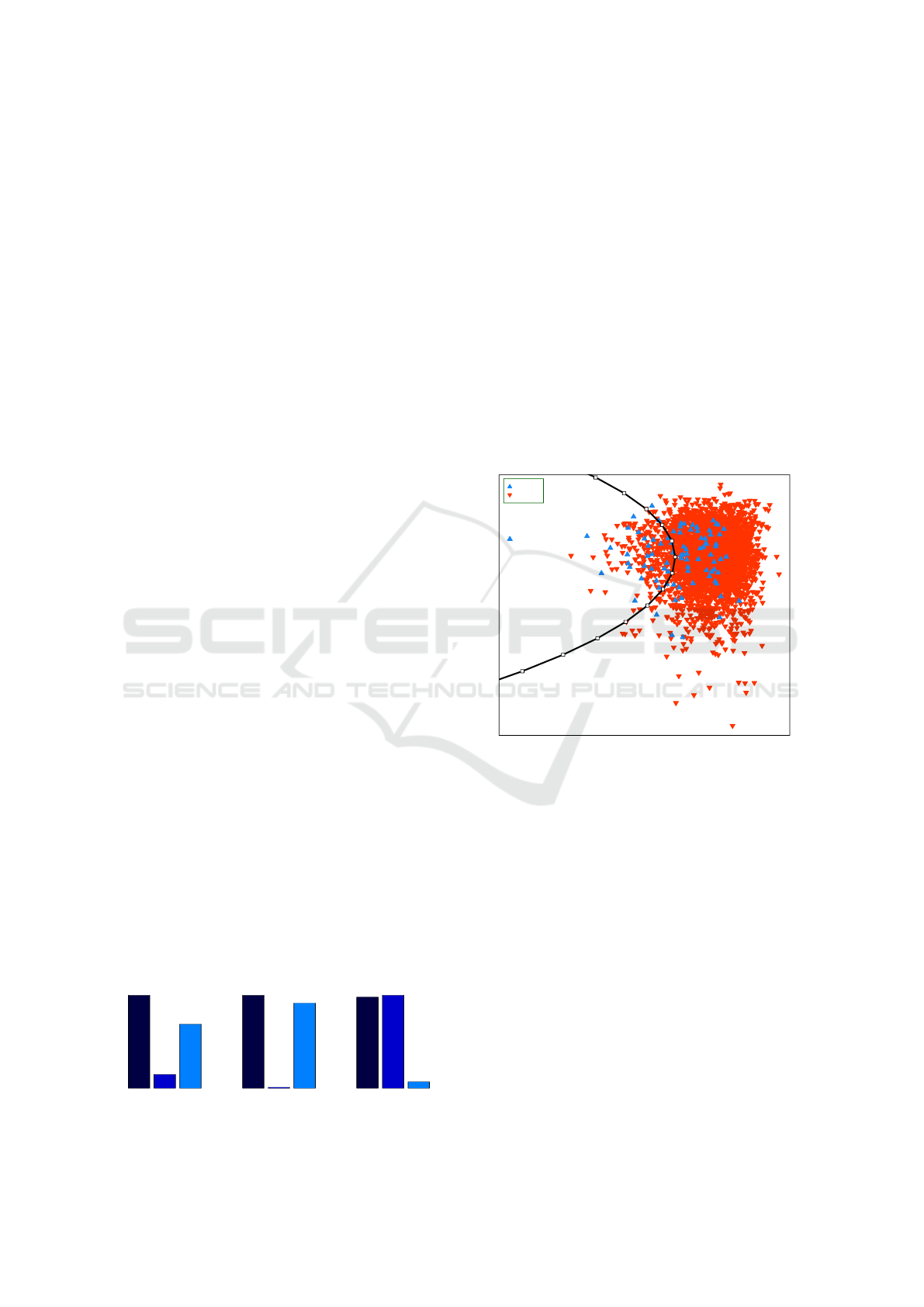
Majority x Minority
Minority
Majority
Figure 3: Two populations of data points overlapping one
another, with an approximately unitary distance between
their barycenters. 97.5% of points belongs to the majority
class, 2.5% to the minority class. A curve decision surface
learned with the SurfOpt Algorithm separates these classes.
5.3 Results
Four classification algorithms were run. The SurfOpt
algorithm was programmed in the R programming
language. For the SVM algorithm, we used the e1071
package (Dimitriadou et al., 2006). For Adabag and
Adaboost, we used the package Adabag (Alfaro et al.,
2013). All the parameters were found with grid-
search. For SurfOpt, we used ω = 0, TNR thresold =
0.35, TPR thresold = 0.10, max iterations = 2000,
resolution = 20. For the AMSmgrad optimization
algorithm, we used α = 0.9, β = 0.9, γ = 0.999.
For the SVM, we used a radial kernel cost = 1000,
γ = 0.1. For the experiments with Adaboost, we used
mfinal = 1 and the Breiman learning coefficient. For
Adabag, we used mfinal = 1, max depth = 70.
ICAART 2019 - 11th International Conference on Agents and Artificial Intelligence
728

Table 1: Mean results for each algorithm.
Algorithm ACC NPV TNR MCC
SurfOpt 88.5% 11% 38.4% 0.156
SVM 97.5% 39.8% 0.7% 0.0409
Adaboost 97.3% 34.5% 7.4% 0.148
Adabag 97.3% 32.8% 8.5% 0.154
Table 1 shows the mean results for 500 synthetic
datasets. Note that the SurfOpt algorithm attains com-
parable performance in terms of mean Matthews Cor-
relation Coefficient (MCC) to the ensemble meth-
ods of Adabag and Adaboost. Support Vector Ma-
chines shows little classification value in terms of
mean MCC. The low mean MCC metric for the SVM
algorithm models can be explained by the fact it is
unable to deal with trade-off regions even with the
radial kernel, as it optimizes for distance to points.
As expected, the skewness made the SVM models bi-
ased to the class with most points. Although SurfOpt
algorithm shows a similar mean MCC to Adaboost
and Adabag ensemble methods, in our algorithm, the
mean True Negative Rate (TNR) is higher than the en-
semble methods, meaning that it correctly predicted a
higher ratio of the negative class data points. With
the observation of those three metrics, it can be iden-
tified the SurfOpt algorithm as a True positive rate
(TPR) detrimental algorithm, as it trades overall ac-
curacy to attain a better classification of the minor-
ity class. SVM, Adaboost and Adabag classifiers are
True Negative Rate (TNR) detrimental, as they only
will predict the minority class if it is a very safe bet.
6 FUTURE WORK
We expect to investigate the properties of an en-
semble approach to the SurfOpt algorithm, using
sets of ununiform curves with complementary opti-
mization criteria, to compensate for individual clas-
sifier’s disadvantages. Other studies may also test
SurfOpt performance regarding oversampling and un-
dersampling approaches, explore the classifier prop-
erties with noisy data, and find a generalization to n-
dimensional spaces.
7 CONCLUSION
In this paper, we have introduced SurfOpt algorithm.
It brings together classification performance with the
benefits of optimizing a classification surface. Op-
posed to common algorithms, SurfOpt algorithm can
better classify the minority class of a binary set even
under severe skewness. We devised a diagnostic to
classification performance for imbalanced data based
on three basic metrics, as an effort to study classifica-
tion under skewness. The source code of this work is
being made avaliable online (Da Silva, 2018).
ACKNOWLEDGMENT
The authors would like to thank the financial support
from CAPES/Brazil and CNPq/Brazil, which was of-
fered through the project Abys (401364/2014-3).
REFERENCES
Alfaro, E., Gamez, M., Garcia, N., et al. (2013). Adabag:
An R Package For Classification with Boosting and
Bagging. Journal of Statistical Software, 54(2):1–35.
Barber, C. B., Dobkin, D. P., and Huhdanpaa, H. (1996).
The Quickhull Algorithm For Convex Hulls. ACM
Transactions on Mathematical Software (TOMS),
22(4):469–483.
Boser, B. E., Guyon, I. M., and Vapnik, V. N. (1992). A
Training Algorithm for Optimal Margin Classifiers. In
Proceedings of the 5th annual workshop on Computa-
tional learning theory, pages 144–152. ACM.
Boughorbel, S., Jarray, F., and El-Anbari, M. (2017).
Optimal Classifier for Imbalanced Data Using
Matthews Correlation Coefficient Metric. PloS one,
12(6):e0177678.
Carneiro, N., Figueira, G., and Costa, M. (2017). A Data
Mining Based System For Credit-Card Fraud Detec-
tion In E-tail. Decision Support Systems, 95:91–101.
Da Silva, A. R. (2018). Surfopt.
https://github.com/andreblumenau/SurfOpt.
Devroye, L. and Toussaint, G. T. (1981). A Note on Linear
Expected Time Algorithms for Finding Convex Hulls.
Computing, 26(4):361–366.
Dimitriadou, E., Hornik, K., Leisch, F., Meyer, D.,
Weingessel, A., and Leisch, M. F. (2006). The e1071
Package. Misc Functions of Department of Statistics
(e1071), TU Wien.
Duchi, J., Hazan, E., and Singer, Y. (2011). Adaptive sub-
gradient methods for online learning and stochastic
optimization. Journal of Machine Learning Research,
12(Jul):2121–2159.
Guo, P., Liu, T., Zhang, Q., Wang, L., Xiao, J., Zhang, Q.,
Luo, G., Li, Z., He, J., Zhang, Y., et al. (2017). Devel-
oping a Dengue Forecast Model using Machine Learn-
ing: A Case Study in China. PLoS neglected tropical
diseases, 11(10):e0005973.
Haixiang, G., Yijing, L., Shang, J., Mingyun, G., Yuanyue,
H., and Bing, G. (2017). Learning from Class-
imbalanced Data: Review of Methods and Applica-
tions. Expert Systems with Applications, 73:220–239.
Hofmann, M. (2006). Support Vector Machines—Kernels
and the Kernel Trick. Notes, 26.
SurfOpt: A New Surface Method for Optimizing the Classification of Imbalanced Dataset
729

Kingma, D. P. and Ba, J. (2015). Adam: A Method For
Stochastic Optimization. 3rd International Confer-
ence for Learning Representations.
Lipton, Z. C., Elkan, C., and Naryanaswamy, B. (2014).
Optimal Thresholding of Classifiers To Maximize F1
Measure. In Joint European Conference on Machine
Learning and Knowledge Discovery in Databases,
pages 225–239. Springer.
Reddi, S. J., Kale, S., and Kumar, S. (2018). On the Conver-
gence of Adam and Beyond. 6th International Con-
ference on Learning Representations (ICLR).
Schapire, R. E. (2013). Explaining Adaboost. In Empirical
inference, pages 37–52. Springer.
Syam, N. and Sharma, A. (2018). Waiting for a Sales Re-
naissance in the Fourth Industrial Revolution: Ma-
chine Learning and Artificial Intelligence in Sales Re-
search and Practice. Industrial Marketing Manage-
ment, 69:135–146.
Zhao, Y., Healy, B. C., Rotstein, D., Guttmann, C. R., Bak-
shi, R., Weiner, H. L., Brodley, C. E., and Chitnis, T.
(2017). Exploration of Machine Learning Techniques
In Predicting Multiple Sclerosis Disease Course. PloS
one, 12(4):e0174866.
ICAART 2019 - 11th International Conference on Agents and Artificial Intelligence
730