Large Neighborhood Search for Periodic Electric Vehicle Routing
Problem
Tayeb Oulad Kouider, Wahiba Ramdane Cherif-Khettaf and Ammar Oulamara
Universit
´
e de Lorraine, Lorraine Research Laboratory in Computer Science and its Applications - LORIA (UMR 7503),
Campus Scientifique, 615 Rue du Jardin Botanique, 54506 Vandœuvre-les-Nancy, France
Keywords:
Periodic Vehicle Routing, Electric Vehicle, Charging Station, Large Neighborhood Search.
Abstract:
In this paper, we address the Periodic Electric Vehicle Routing Problem, named PEVRP. This problem is mo-
tivated by a real-life industrial application and it is defined by a planning horizon of several periods typically
”days”, in which each customer has a set of allowed visit days and must be served once in the time hori-
zon. The whole demand of each customer must be fulfilled all together. A limited fleet of electric vehicles is
available at the depot. The EVs could be charged during their trips at the depot and in the available external
charging stations. The objective of the PEVRP is to minimize the total cost of routing and charging over the
time horizon. We propose a Large Neighborhood Search (LNS) framework for solving the PEVRP. Different
implementation schemes of the proposed method including customer and station insertion strategies, three
destroy operators and three insertion operators are tested on generalized benchmark instances. The compu-
tational results show that LNS produces competitive results compared to results obtained in previous studies.
An analysis of the performance of the proposed operators is also presented.
1 INTRODUCTION
Transport activities are responsible for a significant
part of the world’s greenhouse gas emissions. In order
to reduce these emissions, several initiatives are be-
ing undertaken in the transport sector, particularly for
last-mile activities. Several organisational solutions
have already been implemented, for example, the con-
struction of consolidation centres at the entrance to
cities that allows grouped deliveries. A new orienta-
tion concerns the technological evolution of transport
resources, such as the installation of robot convey-
ors, deliveries by drones, etc. Although these solu-
tions could be viable in the long term, nevertheless,
their large-scale use in the short term raises several
problems, particularly from legislative point of view,
where safety, risk and liability aspects must be identi-
fied.
The electric vehicle has emerged as credible alter-
native solution to reduce carbon emissions in city cen-
tres due to transport activities. Services using electric
vehicles are already deployed to meet the demand of
mobility through several cities. However, from logis-
tic point of view, electric vehicle is still facing weak-
nesses related to the availability of electric vehicles
with an appropriate volume and capacity load for the
large-scale use. Other factors that limited their large-
scale use are mainly their limited driving range, long
charging time, and the availability of a charging in-
frastructure. Despite these weaknesses, in last miles
logistics, the quantities of goods transported, and the
distances covered are fully adapted to the use of elec-
tric vehicles already available on the market.
In this paper, we focus our study on a specific pur-
pose in which electric vehicles are most appropriate,
such as parcel or mail delivery. More precisely, we
consider the periodic electric vehicle routing prob-
lem, in which each client needs only one visit that can
be satisfied according to a set of feasible visit days.
Customers must be assigned to a feasible visit option.
The typical objective is minimizing the total cost in-
cluding charging cost and routing over the planning
period, more details on the problem are provided in
section 3. The rest of the paper is organised as fol-
lows. Section 2 provides a selective review on the
studied problem. Section 3 gives more details on con-
straints and characteristics of our problem. Section 4
proposes solving approaches based on Large Neigh-
borhood Search (LNS). Section 5 presents experimen-
tal results. Section 6 concludes this study with a short
summary and some perspectives.
Kouider, T., Cherif-Khettaf, W. and Oulamara, A.
Large Neighborhood Search for Periodic Electric Vehicle Routing Problem.
DOI: 10.5220/0007409201690178
In Proceedings of the 8th International Conference on Operations Research and Enterprise Systems (ICORES 2019), pages 169-178
ISBN: 978-989-758-352-0
Copyright
c
 2019 by SCITEPRESS – Science and Technology Publications, Lda. All rights reserved
169

2 RELATED WORK
The Periodic Vehicle Routing Problems (PVRP) has
been introduced in (Christofides and Beasley, 1984).
The objective of the PVRP is to find a set of routes
over time horizon of h periods of days that minimizes
total travel time while satisfying vehicle capacity, pre-
determined visit frequency for each client, and spac-
ing constraints. More and more variants of PVRPs
have been proposed in the literature to address real
issues such as the routing of healthcare nurses (Fikar
and Hirsch, 2017), and the transportation of elderly or
disabled persons (Ciss
´
e et al., 2017). Since the PVRP
is NP-Hard problem, most of the methods proposed in
the literature are based on heuristic and metaheuristic
approaches (Mancini, 2016), (Dayarian et al., 2016),
(Baldacci et al., 2011). A survey on the PVRP can be
found in (Francis et al., 2008).
Efficient EV routing is an important management
issue, and a considerable number of papers on sev-
eral variants of EVRP have been published in recent
years.(Schneider et al., 2014) presented the Electric
Vehicle Routing Problem with Time Windows and
Recharging Stations. (Goeke and Schneider, 2015)
addressed the EVRP problem with mixed fleet of
electric and conventional vehicles with time windows
constraints. The heterogeneous electric vehicles con-
straint is considered in (Hiermann et al., 2016). In
(Felipe et al., 2014), the authors present a variation of
the electric vehicle routing problem in which differ-
ent charging technologies and partial EV charging is
allowed. In (Sassi et al., 2015b), (Sassi et al., 2015a)
a rich variant of Electric Vehicles Routing Problem
related to a real application is proposed. This variant
considers a Mixed fleet of conventional and heteroge-
neous electric vehicles and includes different charg-
ing technologies, partial EV charging, compatibility
between vehicles. The charging stations could pro-
pose different charging costs, even if they propose
the same charging technology and they are subject to
operating time windows constraints. The tourist trip
problem for EV with time windows and range limita-
tions is proposed in (Wang et al., 2018). In (Jie et al.,
2019) a variant of two-echelon electric vehicle rout-
ing problem is proposed. (Schiffer and Walther, 2018)
and (Schiffer and Walther, 2017) present a location-
routing approach that considers simultaneous deci-
sions on routing vehicles and locating charging sta-
tions for strategic network design of electric logistics
fleets.
Despite the abundant literature on the EVRP, the
periodic extension of electric vehicles routing prob-
lem has been studied only in (Kouider et al., 2018).
The authors presented a PEVRP (Periodic Electric
Vehicle Routing Problem) variant, which deals with
tactical and operational decisions level for electric ve-
hicles routing and charging, and proposed two con-
structive heuristics to solve the problem. Another
study address the multi-periodic aspect for electric ve-
hicles could be found in (Zhang et al., 2017), but in
this study the routing and the charging over the period
is not considered.
In this paper, we develop a Large Neighborhood
Search for the PEVRP proposed in (Kouider et al.,
2018). Our goal is to enhance the known results. A
classical insertion and destroy operators have been
extended in a non-trivial way to deal with PEVRP
constraints. We propose to study the effectiveness of
these operators in the LNS scheme.
3 PROBLEM DEFINITION
The Periodic Electric Vehicle Routing Problem
(PEVRP) has been introduced in (Kouider et al.,
2018). It is defined on complete directed graph G =
(V, A). V = C ∪B ∪{0} , where 1) the vertex 0 rep-
resents the depot, which contains charging points al-
lowing free charging at night and during the day, 2)
the set C of n vertices represents the customers, for
each customer i a demand q
i
and a service time s
i
are
defined, and 3) the set B of ns vertices denotes the ex-
ternal charging stations, which can be visited during
each day of the planning horizon. A is the arc set with
for each arc (i, j) a travel cost c
i j
, a travel distance d
i j
and a travel time t
i j
. When an arc (i, j) is travelled
by an electric vehicle (EV), it consumes an amount of
energy e
i, j
= r ×d
i, j
, where r denotes a constant en-
ergy consumption rate. This common simplification
of energy consumption is used in the most studies of
the literature on the EVRP. For more details see the
study in (Sassi et al., 2015b).
We consider a time horizon H of np periods typ-
ically ”days”, in which each customer i has a fre-
quency f (i) = 1, and a set of allowed visit days
D(i) ∈ H. This means that customer i must be ser-
viced one time in D(i), and exactly once in the chosen
day.
A fixed charging cost Cc is considered, that nei-
ther depends on the amount of the delivered energy
nor on the time needed to charge the vehicle (Sassi
et al., 2015b) (Sassi et al., 2015a). The amount of
power delivered to each vehicle k at the night of day h
is a decision variable P
h,0,k
, defining the vehicle’s ini-
tial state of charge at the beginning of the trip of the
vehicle k for the day h + 1, h ∈1...np (P
np,0,k
defines
the charging at night for day 1 for the vehicle k).
The PEVRP consists of assigning each client i to
ICORES 2019 - 8th International Conference on Operations Research and Enterprise Systems
170

one service day defined by D(i) that minimize the to-
tal cost of routing and charging over H. A feasible
solution of PEVRP must satisfy the following set of
constraints:
• Each route must start and end at the depot;
• each customer i should be visited once during the
planning horizon, and the visit day must be in
D(i).The customer demand q
i
must be completely
fulfilled during this visit.
• no more than m electric vehicles are used;
• the total duration of each route, calculated as the
sum of (i) travel duration required to visit cus-
tomers, (ii) time required to charge the vehicle
during the day, and (iii) the service time of each
customer; could not exceed T;
• the overall amount of goods delivered along the
route, given by the sum of demands q
i
of visited
customers, must not exceed the vehicle capacity
Q;
The objective function to be minimized is f (x) =
α × f
1
(x) +Cc ×nbs(x) where, f
1
(x) is the total dis-
tance of the solution x over the planning period H, and
nbs(x) is the number of visits to charging stations in
solution x over the planning period, and α is a given
weight representing the cost of one unit of distance.
4 SOLVING APPROACHES
Since the considered problem is NP-hard and in order
to solve large instances of the PEVRP, we develop
a Large Neighborhood Search (LNS) metaheuristic.
LNS was first proposed by (Shaw, 1998), and later
adapted by (Pisinger and Røpke, 2010). The LNS
starts from a given feasible solution and improves it
using the Destroy-Repair strategy. Indeed, LNS re-
moves a relatively large number of customers from
a current solution, and re-inserts these deleted cus-
tomers in different positions. This leads to a com-
pletely different solution, that helps the heuristic to
escape local optima.
In this paper, we propose destroy and repair meth-
ods including specific procedures that are useful to
deal with energy and charging constraints. The first
procedure, named Ad justDecreaseCharging(Tr) is
applied on each modified tour Tr after the ejection
of a certain number of customers by a destroy op-
erator. The purpose of this procedure is to estimate
the unused energy of the modified solution Tr, and
to decide which stations will have to reduce their en-
ergy, or which stations can be removed when station
removal is possible. The second procedure, named
Ad justIncreaseCharging(Tr) is used for each mod-
ified tour Tr after inserting a new customer into the
tour Tr, whose energy is already adjusted. The pur-
pose of this procedure is to estimate the additional en-
ergy to be injected into the modified tour Tr, and to
decide which stations will have to increase their en-
ergy, and/or if necessary which new stations will be
added to the tour Tr. Note that in some cases the al-
gorithm fails to insert an ejected customer i. This can
happen in one of the following cases: 1) the customer
i cannot be inserted into the existing tours because
of the capacity and/or time limit constraints, and no
new tour can be created in any day p of the horizon
because the number of vehicles used in each day p
is equal to m. 2) for each feasible insertion position
given by a day h ∈D(i), a tour t scheduled in the day
h, and a position k ∈t , such that the constraint of ca-
pacity and total time are satisfied but the energy con-
straint is not satisfied for t: there is no charging sta-
tion that can repair t. The next subsections describe
the different LNS procedures in detail.
4.1 Initial Solution Generation
LNS begins by calling one of the two construc-
tion heuristics that we proposed in previous research
(Kouider et al., 2018). The first heuristic, namely BIH
(Best Insertion Heuristic) consists of inserting each
customer i (and when necessary, a charging station b)
at its best position, where a position is characterised
by a day h ∈ D(i), a tour t scheduled in the day h,
and a position k ∈t. The second heuristic is based on
Clustering Analysis, namely CLH (Clustering heuris-
tic). The CLH algorithm proceeds in four steps. The
first step aims at creating m initial clusters in each day,
one for each available vehicle. In the second step, for
each day h, the algorithm CLH tries to dispatch the
maximum number of remaining customers in the m
available clusters of the day y, without inserting any
charging station. In step 3, the customers not inserted
in step 2 due to energy constraint, are considered. In
this step, the objective is minimising the additional
energy consumption for each cluster. Finally, in the
fourth step, a best insertion TSP heuristic is used to
find a feasible route in each cluster for each day.
4.2 Useful Procedures
In this section, we detail some useful procedures that
are needed in different steps of our LNS algorithm.
The Ad justIncreaseCharging(Tr) is used by the in-
sertion operators and Ad justDecreaseCharging(Tr)
is applied to a partial solution after the destroy op-
erator.
Large Neighborhood Search for Periodic Electric Vehicle Routing Problem
171

Let define:
• InitialDepot (respectively EndDepot) : the first
(respectively the last) depot used in a given route
or a given sequence of nodes. InitialDepot and
EndDepot are two distinct copies of the depot d.
• MaxEnergy: the maximum energy that can be
charged in a given station.
• PrecStation(u): return the last charging station
(can be a depot) visited before a node u.
• SuccStation(u): return the first charging station
(can be a depot) visited after a node u.
• GetRecharge(u): return the amount of energy
charged if u is a charging station, 0 else.
• EnergyIn(u): return the amount of energy avail-
able in the vehicle when arriving in the node u.
• EnergyOut(u): return the amount of energy avail-
able in the vehicle when leaving the node u.
• GetMinEnergy(Tr): min
u∈Tr
EnergyIn(u).
• FirstNegativeNode(Tr): by scanning Tr from the
beginning to the end, return the first node u, such
that EnergyIn(u) ≤ 0 or EnergyOut(u) ≤ 0, else
return ∞.
• U pdateCharging(Tr): scan the sequence of Tr
from the InitialDepot to the EndDepot and com-
pute for each node (customers or charging station)
in Tr, the amount of energy EnergyIn(u) to inject
into EV battery upon arriving at each node u, and
the amount of energy EnergyOut(u) in EV battery
when leaving the node u.
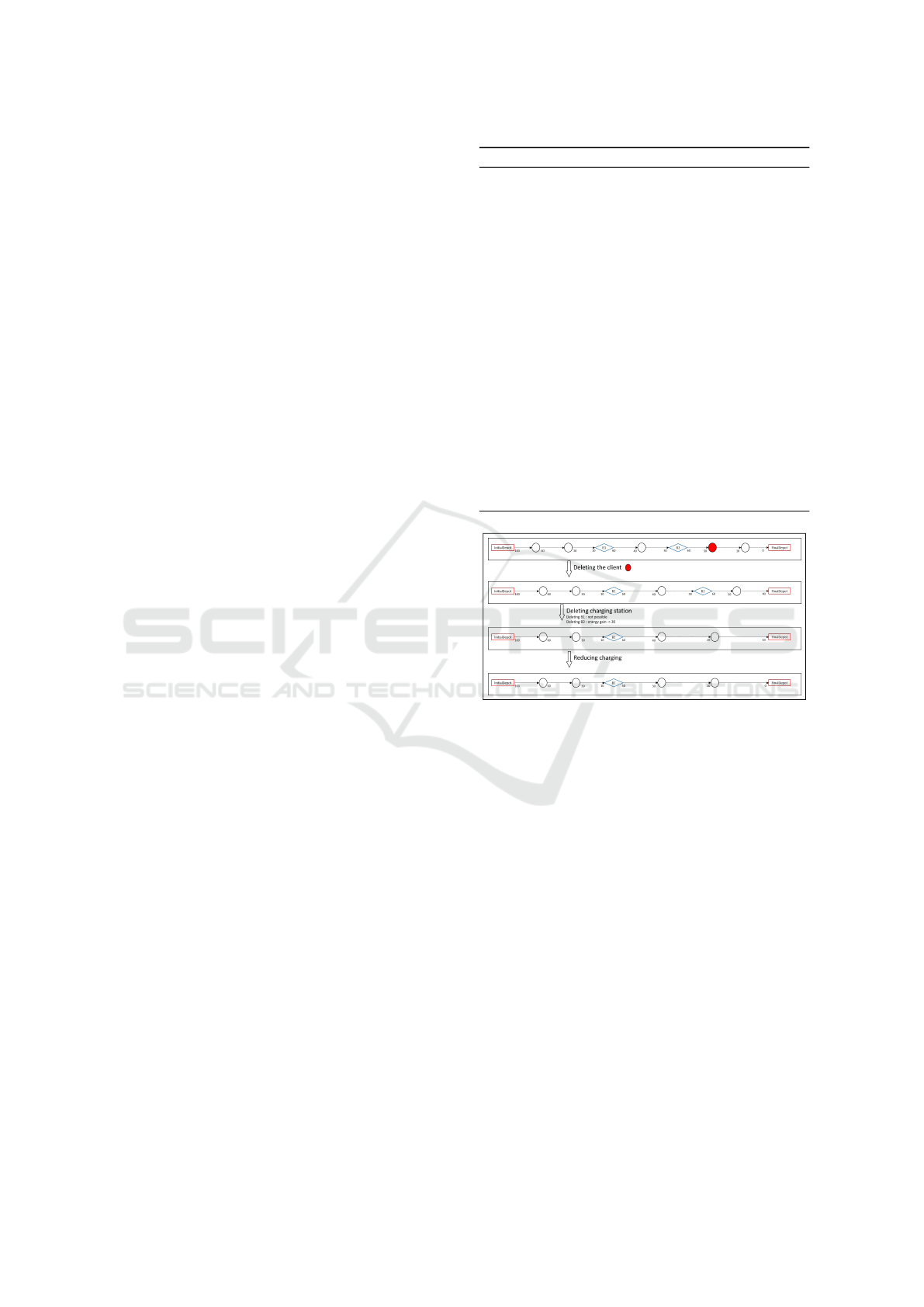
4.2.1 AdjustDecreaseCharging Algorithm
The AdjustDecreaseCharging algorithm (see algo-
rithm 1) receives as an input the sequence Tr after
deleting a set of it customers.
The algorithm repeats the two steps below as long
as EnergyIn(EndDepot) is different from 0. In the
first step, it tries to delete the unused stations, and in
the second step it tries to decrease the energy sup-
plied by each station. A charging station b is unused
if GetRecharge(b) ≤ EnergyIn(SuccStation(b)). In
the first step, as long as there are unused charging sta-
tions in the sequence Tr, the algorithm tries to delete
a station b
∗
, such that b
∗
= argmin
b∈Tr
f (Tr
−b
),
where Tr
−b
denotes a sequence Tr without the sta-
tion b. In the second step the algorithm calls
U pdateCharging(Tr) to adjust the energy (see figure
1).
Algorithm 1: AdjustDecreaseCharging.
1: Input:Sequence Tr after customers removal
2: Output: Updated Tr and f (Tr)
3: while GetMinEnergy(Tr) 6= 0 do
4: u := EndDepot ; v := InitialDepot ;
5: b
∗
= EndDepot ; MinCost := ∞
6: while u 6= v do
7: b := PrecStation(u)
8: if GetRecharge(b) <= EnergyIn(u) then
9: Compute f
0
= f (Tr−b)
10: if f
0
< MinCost then
11: b
∗
← b and MinCost := f
0
12: end if
13: end if
14: u ← b
15: end while
16: if MinCost 6= ∞ then
17: Delete b
∗
; update Tr and f (Tr)
18: end if
19: end while
Figure 1: AdjustDecreaseCharging example.
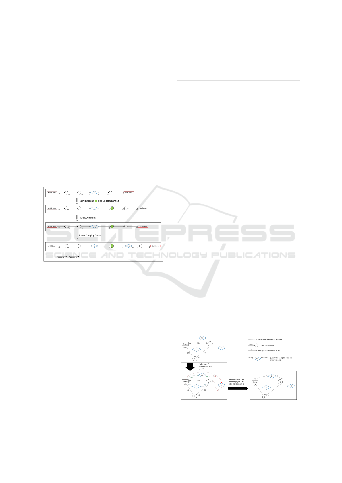
4.2.2 AdjustIncreaseCharging Algorithm
This algorithm is called after the insertion of each
customer. It proceeds in three steps: In the first
one, the procedure U pdateCharging(Tr) is used. If
EnergyIn(u) ≥0 and EnergyOut(u) ≥0, ∀u ∈ Tr, Tr
is still feasible. The algorithm stops and returns the
updated values of EnergyIn and EnergyOut for each
node u ∈ Tr. If ∃u ∈ Tr, such that EnergyIn(u) < 0
or EnergyOut(u) < 0, Tr is unfeasible, then the al-
gorithm proceeds to step 2. Step 2 uses the proce-
dure IncreaseCharging(Tr) to repair the sequence Tr
without adding new stations. It attempts to repair the
route Tr by recharging more energy in stations al-
ready visited in Tr. If the solution becomes feasible,
the algorithm stops and returns the new values of the
energy to be charged in each station, and updates val-
ues of EnergyIn and EnergyOut for each node u ∈Tr.
If Tr stills not feasible, the algorithm runs step 3 and
calls the procedure InsertChargingStation(Tr, b
∗
, k
∗
)
that tries an insertion of charging stations that could
ICORES 2019 - 8th International Conference on Operations Research and Enterprise Systems
172

make the route feasible. More precisely, consider-
ing the sequence Tr from the beginning, let u
−
be
the first node, u ∈ Tr, such that EnergyIn(u) < 0, let
PrecStation(u) = b
−
. Increasing energy after u
−
is
obviously useless. Increasing the energy before b
−
is exactly the same than increasing the amount of en-
ergy to be charged in b
−
knowing that the vehicle has
a limited battery capacity. So, to make the route Tr
feasible in terms of energy, we need to repair the sub-
sequence of nodes between b
−
and u
−
by inserting
new stations. If it is not possible the algorithm stops
and returns ∞. Otherwise the algorithm returns the
station b
∗
to be inserted and the best position k
∗
for
b
∗
. After inserting b
∗
in Tr, the U pdateCharging(Tr)
procedure is applied to update the values of EnergyIn
and EnergyOut. The algorithm repeats the procedure
InsertChargingStation(Tr, b
∗
, k
∗
) as long as there are
negative nodes and inserting charging stations is pos-
sible. See Figure 2.
Figure 2: AdjustIncreaseCharging example.
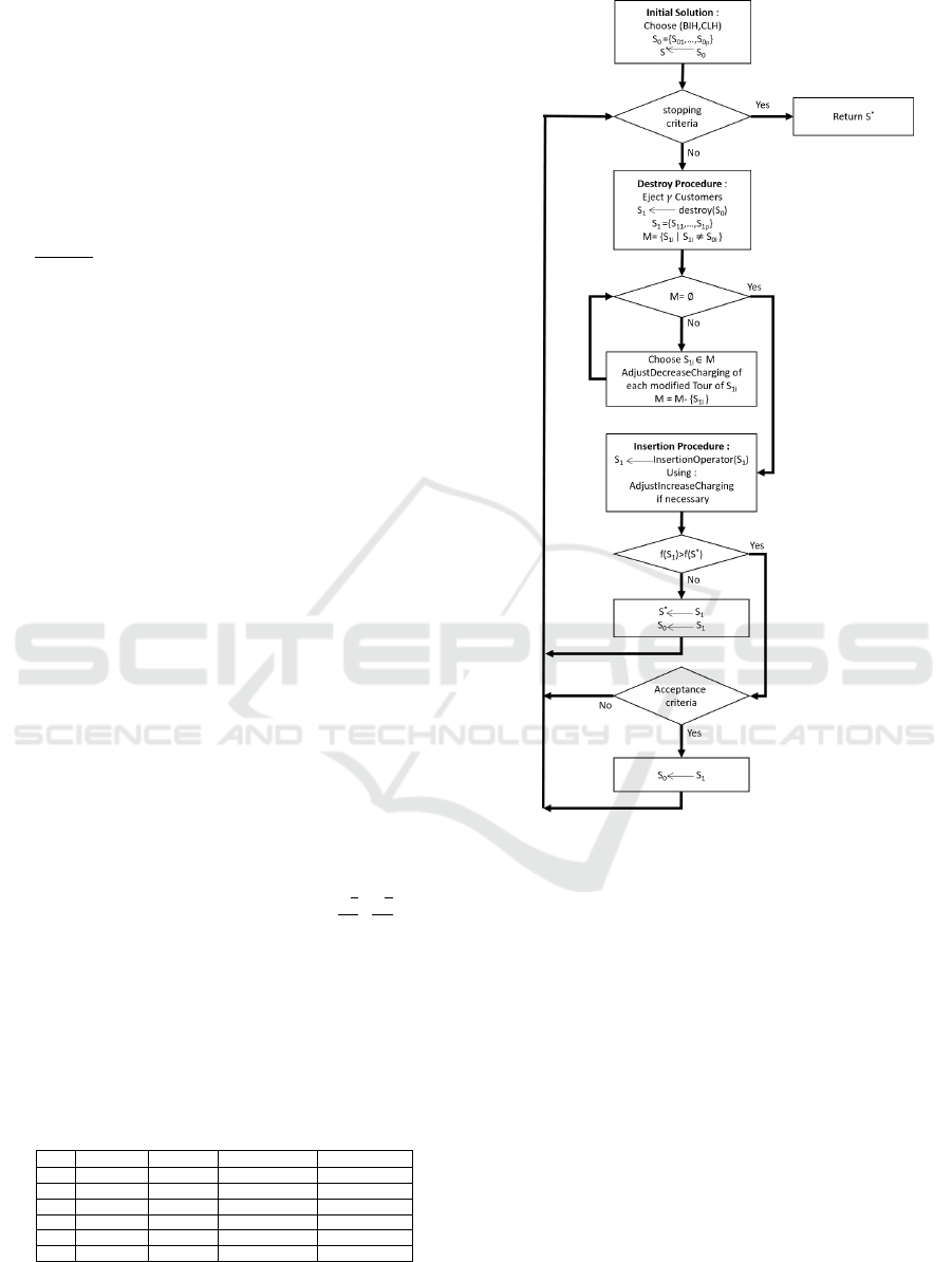
In InsertChargingStation(Tr, b
∗
, k
∗
) method, we
propose two techniques for selecting the station to be
inserted ; the first one, named InsertS
all
, tries the in-
sertion of all charging stations in all positions between
b
−
and u
−
, and chooses the insertion that repair the
route with the lower cost. The second method, named
InsertS
1
, choose, for each position k between b
−
and
u
−
, the charging station b
0
that gives the highest gain
of energy to the route and test the insertion, i.e., b
0
=
argmin
b∈B
{e
b,succ(k)
|(EnergyOut(k) − e
k,b
) > 0},
such that succ(k) represents the node located directly
after the position k in the route. Among all positions
that have been tested we choose the one with the
lower cost. In the Figure 3, we give an example
of the first iteration of InsertS
1
. In that example,
b
−
= Depot and u
−
= 2. So we need to test the
insertion of charging stations between the Depot and
the customer 1 and between the customer 1 and the
customer 2 in order to select the lowest cost feasible
insertion. For example, between the Depot and the
customer 1, while InsertS
all
simulates and tests the
insertion of all stations, here b1, b2, and b3 ; InsertS
1
simulates and tests only the insertion of b1.
Algorithm 2: AdjustIncreaseCharging.
1: Input:sequence Tr after the insertion of customer
i
2: Output: ∞ if Tr is unfeasible, else the updated
Tr and f (Tr)
3: b
∗
= k
∗
= 0,
4: Step 1: U pdateCharging(Tr)
5: u
−
:= f irstNegativeNode(Tr)
6: if (u
−
= ∞) then
7: Go to 30
8: else
9: b
−
:=PrecStation(u
−
)
10: Go to 11
11: end if
12: Step 2: IncreaseCharging(Tr)
13: if (EnergyOut(b
−
) 6= MaxEnergy) then
14: Go to 18
15: else
16: Go to 23
17: end if
18: if (MaxEnergy − EnergyOut(b
−
)) ≥
GetMinEnergy(Tr) then
19: Increase the recharge of b
−
by
(GetMinEnergy(Tr)), Go to 30
20: else
21: Increase the recharge of b
−
by (MaxEnergy−
EnergyOut(b
−
)), Go to 4
22: end if
23: Step 3 : InsertChargingStation(Tr, b
∗
, k
∗
)
24: if (b
∗
= k
∗
= 0) then
25: return ∞
26: else
27: Go to 26
28: end if
29: Insert b
∗
in k
∗
, update Tr.
30: return the updated Tr, and f (Tr)
Figure 3: Charging station insertion.
Large Neighborhood Search for Periodic Electric Vehicle Routing Problem
173

4.3 Destroy Operators
The destroy operators remove a given number of cus-
tomers (denoted γ) from a current solution. We pro-
pose three destroy operators inspired from the re-
movals operators presented in (Pisinger and Røpke,
2010). They consist in the random removal, the worst
removal, and the cluster removal. In the following,
we give a description of these operators. Let S =
{S
1
, .., S
np
} the initial feasible solution, and S
h
a set
of routes in the day h, S
h
= {T
1h
. . . T
kh
..T
mh
}. After
removing γ customers, a new partial solution S
0
is gen-
erated. S
0
= {T
0
1h
. . . T
0
kh
, .., T
0
mh
}, such that T
0
kh
= T
kh
if
no customer has been deleted from T
kh
, and T
0
kh
= T
−
kh
if one or more customers has been deleted from T
kh
.
4.3.1 Random Removal (S, S
0
, f (S
0
))
This operator randomly removes γ cus-
tomers from the solution. The procedure
Ad justDecreaseCharging(Tr) is applied to each
trip T
−
kp
∈ S
0
. The new cost of the partial solution
f (S
0
) is returned.
4.3.2 Cluster Removal (S, S
0
, f (S
0
))
This operator starts by randomly choosing a cus-
tomer i, then γ −1 additional customers located near-
est to i (in terms of costs) are selected (the selected
neighbours may be in different routes and differ-
ent days and are not necessary in trip(i), such that
trip(i) gives the tour that include i). The proce-
dure Ad justDecreaseCharging(Tr) is applied to each
route T
−
kp
∈ S
0
. The new cost of the partial solution
f (S
0
) is returned.
4.3.3 Worst Removal (S, S
0
, f (S
0
))
For each customer i ∈ S, the algorithm simulates the
removal of i, by deleting i from S, and applying
Ad justDecreaseCharging(trip(i)
−i
). The total cost
f (S
0−i
) is computed for each removal simulation. The
customers i
∗
whose removal produces the biggest de-
crease in the objective function is chosen. This algo-
rithm stops when γ customers was deleted.
4.4 Insertion Operators
We have implemented three insertion op-
erators, namely, First Improvement, Best
Improvement, Regret Insertion. we apply
Ad justIncreaseCharging(Tr) to adjust the charging
of each modified tour Tr ∈ S. If it’s not possible to
insert an ejected node in an already constructed route,
a new route that contains this node and the depot may
be created if the number of used vehicles is less than
m. When all customers have been reinserted back
into the solution using a predefined insertion method,
the new solution is compared with the original
solution. The solution may become unfeasible if it is
impossible to insert all ejected clients. To limit the
insertion positions to be tested before inserting one
customer i, two insertion strategies are proposed. The
first strategy, named InsertC
All
, tests all insertion
positions in Tr, the number of positions to be tested
is |Tr|−1. In the second strategy, named InsertC
α
,
α nodes u
1
. . . u
α
closest to i in terms of distance are
selected. The insertion positions held are then the
positions before and after each selected node.
4.4.1 First Improvement Insertion
This method selects randomly a node among the list
L of ejected nodes and inserts it in the position that
generates the minimal cost increase. If the insertion
of a customer i in a given position of a route t leads to
a violation of the vehicle capacity or total time con-
straints, this route position will not be accepted. How-
ever, if the insertion of a customer in a given route po-
sition still satisfies the vehicle capacity and total time
constraints but leads a violation of the energy con-
straints (in the case where the EV needs more energy
to serve this customer), Ad justIncreaseCharging(t)
is applied to repair the solution. At each update of the
routing and charging solution, the total solution cost
is updated.
4.4.2 Best Improvement Insertion
Let L be the list of ejected customers. This proce-
dure repeats the three steps below until L =
/
0. Step
1 computes the minimum cost insertion of each cus-
tomers i ∈ L using Ad justIncreaseCharging(Tr) if
necessary. In step 2, the customer i
∗
(and eventually
the charging station b
∗
) with the minimum insertion
cost is inserted at its best position, and finally in step
3 L and S are updated.
4.4.3 Regret Insertion
Let L be the list of ejected customers. This proce-
dure repeats the three steps below until L =
/
0. Step1
computes the difference between the two best cost in-
sertions of each customers i ∈ L, denoted δ
i
. if the
insertion of a customer in a given route position sat-
isfies the vehicle capacity and total time constraints
but leads to a violation of the energy constraints,
Ad justIncreaseCharging(Tr) is applied to repair the
solution. In Step 2, a customer i
∗
(and eventually the
ICORES 2019 - 8th International Conference on Operations Research and Enterprise Systems
174

charging station b
∗
) with the maximum δ
i
∗
is inserted
at its best position. Step 3 update L and S.
4.5 Acceptance Criteria
We propose to use the Simulated Annealing principle
as acceptance criteria. Hence, a solution is accepted
if it is better than the best or the current solutions or,
if the metropolis rule is satisfied. In other words, bad
solutions are accepted with the probability given by
exp
f (s)−f (s
0
)
T
, where f (.) stands for the objective func-
tion, s
0
and s are the new and the current solutions
respectively, and T > 0 denotes the current tempera-
ture. At each iteration, the current temperature T is
decreased using the cooling rate c ∈]0, 1[ according to
the expression T = T ×c. We decide to initialise the
temperature in a way that at first iterations of LNS, a
solution 20% worse than the current one will be ac-
cepted with probability of 0.5. The cooling rate is
initialised to 0.9995.
Figure 4 presents the general framework of the
proposed LNS metaheuristic.
5 COMPUTATIONAL
EXPERIMENTS
Our methods are implemented using C++. All com-
putations are carried out on an Intel Core (TM) i7-
5600U CPU, 2.60 GHz processor, with 8GB RAM
memory. We conducted numerical experiments on
PEVRP Benchmark Instances proposed in (Kouider
et al., 2018). These instances are inspired by the
data instances provided by (Felipe et al., 2014). Each
PEVRP instance is composed of n customers and five
or nine charging stations. The number of vehicles
is generated randomly in the interval [
√
n
4
,
√
n
2
]. The
other setting parameters of our instances can be found
in (Kouider et al., 2018). In this paper, we present re-
sults on 9 instances with 100 clients. After several
tests using different parameters, we decide to set the
number of iterations to 1000 and the number of clients
to reject γ = 20.
Table 1: The influence of customer and station insertion
strategies on LNS results.
InsertC
α
InsertS
β
Improvement CPU (hours)
v1 α = 2 β = 1 15,4% 2,5
v2 α = 2 β = all 14,3% 2,5
v3 α = 3 β = 1 15,3% 2,8
v4 α = 3 β = all 15,8% 2,9
v5 α = all β = 1 15,5% 3,0
v6 α = all β = all 16,0% 3,0
In the first tests summarized in table 1, we ex-
amine whether the insertion strategies of customers
Figure 4: LNS scheme.
and charging stations have an influence on the quality
of the solution and the computing time. We tested 6
versions of LNS, named v1 to v6 obtained by fixing
the number of insertion positions α = {2, 3, all} and
β = {1, all}. For each version, we performed 32 tests
on all instances by varying the LNS operators and the
initial solution. We compute in column 4 the aver-
age improvement of LNS on all tests compared to the
initial solution (BIH or CLH). The average CPU time
is indicated in column 5. Table 1 shows that the dif-
ference between the results obtained for each version
of LNS is not important. The average improvement
varies from 14.3% to 16% and the average time from
2.5h to 3h. Compared to the v6 version where we test
all possible positions and the v2 version (which gets
the worst improvement), we get a gain of 0.5 hours
computing time against a loss of 1.7% in improve-
ment. We then decided for the rest of the experiments,
to continue to vary α and β.
Large Neighborhood Search for Periodic Electric Vehicle Routing Problem
175

To compare the performance of the destroy and in-
sertion operators proposed in section 4, we evaluated
the LNS results by testing all operator pairs (table 2
and figure 5). For each choice of operator pair (a line
in Table 2), we compute the average result obtained
on all instances by varying the initial solution, α and
β. The results clearly show that the random destroy
operator is the most efficient (LNS with the random
destroy operator obtains on average 22% to 28% im-
provements compared to the initial solution). The ran-
dom destroy operator allows for a better diversifica-
tion of the solution. It increases the chance of finding
better insertions for the ejected customers. The clus-
ter operator that gives the worst results, ejects cus-
tomers who are close enough. As a result, whatever
the insertion operator used, the cluster destroy opera-
tor has more difficulty to find better insertions for the
ejected customers. The insertion operator ”Regret”
gives the best results regardless of the destroy opera-
tor. The operators ”First Improvement insertion” and
”Best Improvement insertion” give almost similar re-
sults in terms of quality, but the computing time of
”Best Improvement insertion” is about twice the com-
puting time of ”First Improvement insertion”.
Table 2: Evaluation of destroy and insertion operators.
Destroy
operators
Insertion
operators
Improvement CPU (hours)
Cluster Best Imp 8% 2,1
Cluster First Imp 9% 1,0
Cluster Regret 13% 2,6
Random Best Imp 22% 2,2
Random First Imp 23% 1,0
Random Regret 28% 2,9
Worst Best Imp 13% 3,9
Worst First Imp 13% 2,1
Worst Regret 15% 3,7
Figure 5: Evaluation of destroy and insertion operators.
In table 3, we detail the results for the best pairs
of operators. We choose the random destroy opera-
tor and the two insertion operators ”regret” and ”first
improvement”. We note LNS1 the version of LNS
using the operator pair (random, first improvement),
and LNS2 the LNS version using the pair (random, re-
gret). Column 2 (respectively column 5) gives the ini-
tial solution obtained with BIH (respectively CLH).
Column 3 and 4 (respectively column 6 and 7) gives
the Gap of LNS solution in relation to the BIH ini-
tial solution (respectively CLH initial solution). For a
given instance, we note in bold the best solution found
(Best Cost). The results show that LNS can improve
the initial solution on average by up to 34%. LNS
succeeds in improving the initial solution in all cases
except in the instance 3. The best solution is obtained
in 2 cases by LNS2 using CLH as initial solution, and
in 6 cases by LNS2 using BIH. We can conclude that
LNS using the initial solution BIH and the destroy op-
erator Random and the insertion operator regret gives
the best performance.
Table 3: Computational results of LNS with random destroy
operator and regret insertion operator.
BIH CLH
S
0
Cost
LNS1
Gap
S0
LNS2
Gap
S0
S
0
Cost
LNS1
Gap
S0
LNS2
Gap
S0
Best
Cost
Inst1 1600,28 0% 8% 2050,72 21% 29% 1466,23
Inst2 1543,80 0% 0% 2062,29 20% 25% 1539,83
Inst3 1596,50 0% 0% 2260,59 23% 27% 1596,50
Inst4 3798,70 54% 57% 4543,74 62% 63% 1642,74
Inst5 3247,57 35% 43% 3476,44 40% 43% 1842,20
Inst6 2751,84 24% 31% 2818,55 27% 29% 1906,10
Inst7 2491,52 19% 27% 2663,88 25% 29% 1816,03
Inst8 2826,77 23% 28% 3219,18 33% 33% 2042,13
Inst9 2836,07 26% 29% 2825,21 24% 28% 2008,86
Avg 20% 25% 30% 34%
In table 4, we calculated at each 250 iterations, the
number of new best solutions found. More precisely,
for each interval we calculate the average on all in-
stances of the number of times the best solution was
reached. The values are not cumulative, i.e. if the best
solution is reached in one interval, we do not consider
this solution in the other intervals. We only consider
the new best solutions that will be obtained in the con-
cerned interval. The results reveal that about half of
the best solutions are found between 0 and 500 and
that between 750 and 1000 iterations the percentage
of the best solutions found is not negligible. Follow-
ing these results, we decide to examine whether the
percentage of improvement is significant enough.In
figure 6, we show for each version of LNS studied
in table 3 and table 4 the evolution curve of the av-
erage gap in relation to the initial solution on all in-
stances using the results obtained at the end of each
iteration 250, 500, 750 and 1000. We note that the
convergence is almost achieved at iteration 250 and
that after 250 iterations the improvement is very small
Table 4: Percentage of the number of best solutions found
each 250 iterations.
Iterations
0 ]0,250] ]250,500] ]500,750] ]750,1000]
BIH+LNS(1 imp) 33% 0% 33% 0% 33%
BIH+LNS(Regret) 22% 11% 11% 11% 44%
CLH+LNS(1 imp) 0% 22% 22% 33% 22%
CLH+LNS(Regret) 0% 0% 33% 22% 44%
ICORES 2019 - 8th International Conference on Operations Research and Enterprise Systems
176

Figure 6: Evolution of the average gap for four LNS vari-
ants.
therefore running the LNS for 250 iterations is a good
compromise to reduce the execution time.
6 CONCLUSION
In this paper, we considered a Periodic Electric Ve-
hicle routing problem. This problem consists in op-
timizing the routing and charging of a fixed set of
vehicles over a multi-period horizon. To solve this
problem, we developed a Large Neighborhood Search
metaheuristic. We proposed three destroy and three
insertion operators. These operators use specific pro-
cedures to deal with energy and charging constraints.
Nine variants of LNS have been tested by varying
the operators. Preliminary results show the effective-
ness of LNS since it can improve heuristic methods
proposed in previous research by 34% on average.
The results also show that the best performance was
achieved with the random destroy operator and the re-
gret insertion operator. The computation time remains
important but we have shown that reducing the num-
ber of iterations from 1000 to 250 does not deteriorate
significantly the quality of the obtained solutions. As
further work, we will intensify the experiments using
other instances. We are also interested in studying the
influence of the proposed destroy and insertion op-
erators in an Adaptive Large Neighborhood Search
(ALNS) framework and evaluating the performance
of ALNS on PEVRP.
REFERENCES
Baldacci, R., Bartolini, E., Mingozzi, A., and Valletta, A.
(2011). An exact algorithm for the period routing
problem. Operations research, 59(1):228–241.
Christofides and Beasley, J. (1984). The period routing
problem. Networks, 14:237–256.
Ciss
´
e, M., Yalc¸ında
˘
g, S., Kergosien, Y., S¸ahin, E., Lent
´
e,
C., and Matta, A. (2017). Or problems related to home
health care: A review of relevant routing and schedul-
ing problems. Operations Research for Health Care,
13-14:1 – 22.
Dayarian, I., Crainic, T., Gendreau, M., and Rei, W. (2016).
An adaptive large-neighborhood search heuristic for a
multi- period vehicle routing problem. Transportation
Research Part E, 95:95–123.
Felipe, M., Ortuno, T., Righini, G., and Tirado, G. (2014). A
heuristic approach for the green vehicle routing prob-
lem with multiple technologies and partial recharges.
Transportation Research Part E: Logistics and Trans-
portation Review, 71:111–128.
Fikar, C. and Hirsch, P. (2017). Home health care routing
and scheduling: A review. Computers & Operations
Research, 77:86 – 95.
Francis, P., Smilowitz, K., and Tzur, M. (2008). The Vehi-
cle Routing Problem: Latest Advances and New Chal-
lenges, volume 43, chapter The period vehicle routing
problem and its extensions. Springer.
Goeke, D. and Schneider, M. (2015). Routing a mixed fleet
of electric and conventional vehicles. European Jour-
nal of Operational Research, 245(1):81–99.
Hiermann, G., Puchinger, J., Ropke, S., and Hartl, R.
(2016). The electric fleet size and mix vehicle rout-
ing problem with time windows and recharging sta-
tions. European Journal of Operational Research,
252(3):995–1018.
Jie, W., Yang, J., Zhang, M., and Huang, Y. (2019). The
two-echelon capacitated electric vehicle routing prob-
lem with battery swapping stations: Formulation and
efficient methodology. European Journal of Opera-
tional Research, 272(3):879 – 904.
Kouider, T. O., Ramdane-Cherif-Khettaf, W., and Oula-
mara, A. (2018). Constructive heuristics for periodic
electric vehicle routing problem. In Proceedings of the
7th International Conference on Operations Research
and Enterprise Systems - Volume 1: ICORES,, pages
264–271. INSTICC, SciTePress.
Mancini, S. (2016). A real-life multi depot multi period
vehicle routing problem with a heterogeneous fleet:
Formulation and adaptive large neighborhood search
based matheuristic. Transportation Research Part C,
70:100–112.
Pisinger, D. and Røpke, S. (2010). Large Neighborhood
Search, pages 399–420. Springer, 2 edition.
Sassi, O., Ramdane-Cherif-Khettaf, W., and Oulamara, A.
(2015a). Iterated tabu search for the mix fleet vehi-
cle routing problem with heterogenous electric vehi-
cles. Advances in Intelligent Systems and Computing,
359:57–68.
Sassi, O., Ramdane-Cherif-Khettaf, W., and Oulamara, A.
(2015b). Multi-start iterated local search for the mixed
fleet vehicle routing problem with heterogeneous elec-
tric vehicles and time-dependent charging costs. Lec-
ture Notes in Computer Science, 9026:138–149.
Large Neighborhood Search for Periodic Electric Vehicle Routing Problem
177

Schiffer, M. and Walther, G. (2017). The electric loca-
tion routing problem with time windows and partial
recharging. European Journal of Operational Re-
search, 260:995–1013.
Schiffer, M. and Walther, G. (2018). Strategic planning
of electric logistics fleet networks: A robust location-
routing approach. Omega, 80:31 – 42.
Schneider, M., Stenger, A., and Goeke, D. (2014). The elec-
tric vehicle routing problem with time windows and
recharging stations. Transportation science, 75:500–
520.
Shaw, P. (1998). Using constraint programming and local
search methods to solve vehicle routing problems. In
Maher, M. and Puget, J.-F., editors, Principles and
Practice of Constraint Programming — CP98, pages
417–431, Berlin, Heidelberg. Springer Berlin Heidel-
berg.
Wang, Y.-W., Lin, C.-C., and Lee, T.-J. (2018). Electric
vehicle tour planning. Transportation Research Part
D: Transport and Environment, 63:121 – 136.
Zhang, A., Kang, J. J. E., and Kwon, C. C. (2017). Incorpo-
rating demand dynamics in multi-period capacitated
fast-charging location planning for electric vehicles.
Transportation Research Part B, 103:5–29.
ICORES 2019 - 8th International Conference on Operations Research and Enterprise Systems
178