Performance Characterization of Absolute Scale Computation for 3D

Structure from Motion Reconstruction

Ivan Nikolov and Claus Madsen

Department of Architecture, Design and Media Technology, Aalborg University, Rendsburggade 14, Aalborg, Denmark

Keywords:

Scaling, 3D Reconstruction, Structure from Motion (SfM), GPS, Robustness.

Abstract:

Structure from Motion (SfM) 3D reconstruction of objects and environments has become a go-to process,

when detailed digitization and visualization is needed in the energy and production industry, medicine, culture

and media. A successful reconstruction must properly capture the 3D information and it must scale everything

to the correct scale. SfM has an inherent ambivalence to the scale of the scanned objects, so additional

data is needed. In this paper we propose a lightweight solution for computation of absolute scale of 3D

reconstructions by using only a real-time kinematic (RTK) GPS, in comparison to other custom solutions,

which require multiple sensor fusion. Additionally, our solution estimates the noise sensitivity of the calculated

scale, depending on the precision of the positioning sensor. We ﬁrst test our solution with synthetic data to

ﬁnd how the results depend on changes to the capturing setup. We then test our pipeline using real world data,

against the built-in solutions used in two state-of-the-art reconstruction software. We show that our solution

gives better results, than both state-of-the-art solutions.

1 INTRODUCTION

1.1 Object 3D Reconstruction

With the emergence of more and more powerful CPU

and GPUs, SfM software solutions have become wi-

despread and easier to use. This gives both more spe-

cialized industry, medicine and culture preservation

users the possibility to quickly capture objects and en-

vironments. Due to the nature of SfM, to create a de-

tailed reconstruction of both object and texture, users

need only a camera and the software. This gives SfM

solutions the edge, compared to other low-cost 3D re-

construction solutions, like the ones based on time-

of-ﬂight (Corti et al., 2016), structured light (Sarbo-

landi et al., 2015) or stereo cameras (Sarker et al.,

2017). These solutions require appropriate hardware,

together with the specialized software, which gives

them a larger overhead, for users to get into. Exam-

ples of 3D reconstruction using these methods are ex-

tensively benchmarked by (Jamaluddin et al., 2017),

(Sch

oning and Heidemann, 2016).

1.2 State of the Art

An important requirement for the state of the art SfM

software is for it to be both versatile and robust. This

is especially true for images taken in environments

with varying conditions and containing objects with

different shapes and sizes. Many of the state of the art

SfM solutions fall in the category of open-source soft-

ware like OpenSfM (VisualSFM, 2011), COLMAP

(Schonberger, 2016), etc. Other SfM solutions are de-

veloped as part of commercial products like Contex-

tCapture (Bentley, 2016), PhotoScan (Agisoft, 2010)

and RealityCapture (CapturingReality, 2016). All of

these solutions contain a whole processing pipeline

going from the input images to a dense point cloud

and mesh. One drawback that SfM has, is the am-

biguity of the scale of the reconstructed object. The

2D information extracted from images, does not al-

low determining of the absolute scale of the scanned

object. For obtaining this essential information, ad-

ditional information is needed from the user or from

external sensors.

This is why the programs also contain different

built-in solutions for scaling the ﬁnal model. In most

cases these solutions are either using markers or ma-

nual distance measurement. This works only when

there is access to the reconstructed objects or surfa-

ces. This means that they are unfeasible for scanning

structures with drones or scanning hard to reach or

dangerous places. Another method is using the GPS

positions for ﬁnding the absolute scale of the object,

884

Nikolov, I. and Madsen, C.

Performance Characterization of Absolute Scale Computation for 3D Structure from Motion Reconstruction.

DOI: 10.5220/0007444208840891

In Proceedings of the 14th International Joint Conference on Computer Vision, Imaging and Computer Graphics Theory and Applications (VISIGRAPP 2019), pages 884-891

ISBN: 978-989-758-354-4

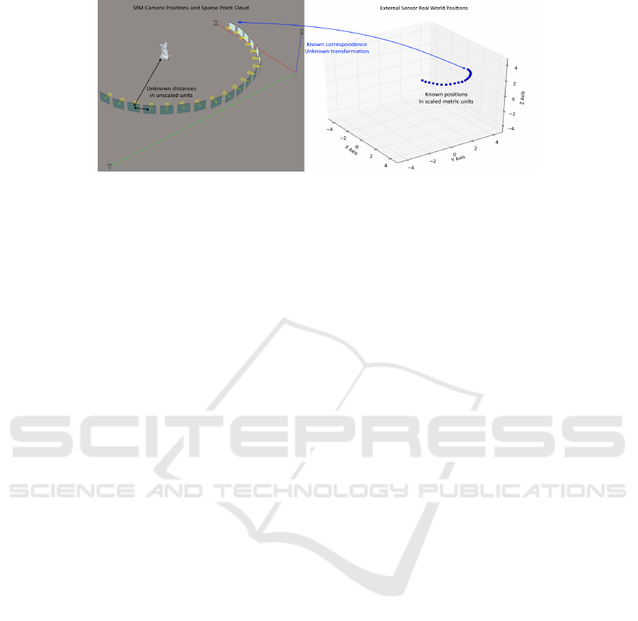
Figure 1: The two sets of corresponding points. On the left an output screen from 3D reconstruction program with the camera

positions and a sparse point cloud, with unknown scale. On the right the same camera positions in a scaled real world metric

units from an external sensor. Establishing the absolute scale of the reconstruction involves estimation the transformation,

which will transfer the left set of points to the right.

but this way does not characterize the performance of

the scaling and do not take into consideration exter-

nal factors, which can inﬂuence the precision of the

scaling.

1.3 Using External Sensor Data for

Determining Scale and Noise

Sensitivity

We propose a solution for determining the absolute

scale for 3D SfM reconstructions using GPS posi-

tioning information, enhanced by RTK for a more

precise estimation of the camera for each image ta-

ken. Others have proposed method for using GPS

and RTK (Rabah et al., 2018), (Dugan, 2018) for ge-

oreferencing and enchanting the SfM reconstruction

workﬂow, but they do not focus on the scale of the

reconstructed objects. Our method is aimed at being

used as part of a unmanned aerial vehicle (UAV) so-

lution for scanning and 3D reconstruction of hard to

reach surfaces and objects. It also works only with

GPS data, in contrast with other methods using sen-

sor fusion (Sch

ops et al., 2015). As the method is ai-

med for industrial and historical preservation use, not

only is the absolute scale needed, but also calculating

the uncertainty of said scale, as well as determining

how capturing conditions and external factors might

inﬂuence it. As an example, we show that when you

have 3 captured horizontally spaced camera positi-

ons from the reconstruction process, a scaled distance

of 100mm on a reconstructed object can be with un-

certainty of 0.1mm. While the same scaled distance,

when calculated from 18 captured horizontally spaced

camera positions has uncertainty of 0.007mm.

Our main contribution is this combination of esti-

mating the absolute scale and its sensitivity to noise,

which in the end gives both precise and robust results.

To test our approach, we ﬁrst analyze the sensor

and determine its accuracy and precision. We then

do a series of simulated test scenarios to get a base-

line of the expected performance. Finally, we test the

method in a real world testing scenario and compare

results to the scaling results produced by the two 3D

reconstruction programs - ContextCapture and Pho-

toScan. We demonstrate that our method gives better

results than the state-of-the-art, while also providing

a reliable uncertainty metric.

2 METHODOLOGY

2.1 SfM Pipeline

To understand the proposed workﬂow, the SfM pi-

peline needs to be ﬁrst explored. SfM relies on in-

formation captured from multiple images around the

scanned objects. Features are extracted from each

image and matched. Normally algorithms like SIFT

(Lowe, 2004), SURF (Bay et al., 2006) are used.

From these matched points a sparse 3D point cloud

can be triangulated using bundle adjustment (Triggs

et al., 1999) and the camera positions can be back-

projected. From these a dense point cloud and subse-

quent mesh can be created. The problem is that there

is no information in 2D images alone on how big the

scanned object is - is it a city or a model of a city?

This is also reﬂected in the calculated camera positi-

ons.

2.2 Least-squares Transformation

Estimation

When capturing the images, the positions of the ca-

meras can be saved in real world coordinates. The

GPS-RTK can be directly positioned on the camera

or on a drone caring the camera. To calculate the real

Performance Characterization of Absolute Scale Computation for 3D Structure from Motion Reconstruction

885

world scale of the reconstruction, the transformation

between the two sets of coordinates needs to be de-

termined - the ones calculated by the SfM software

and the ones given by the GPS-RTK. This is shown in

Figure1, where an output of SfM software is shown

on the left side and the GPS-RTK points are shown

on the right side.

Because there is clear a correspondence between

the SfM camera positions and the GPS-RTK posi-

tions and the unknown transformation consists only

of translation, rotation and uniform scaling, a sim-

ple least-squares estimation algorithm is conside-

red. An implementation of the classical algorithm by

(Umeyama, 1991) is chosen and customized for the

needs of the paper. For the algorithm to work the two

point sets need to have non-collinear points and no

outliers.

We need to also take into consideration the pro-

blem of the lever-arm offset between the GPS antenna

and the camera (Daakir et al., 2016). As an initial ca-

libration step the real-world distance between the two

is measured and used as an additional input for the

Least-Squares estimation algorithm.

= T (b

), a

∈ A, b

∈ B (1)

T =







+ x

o f f

+ y

o f f

+ z

o f f

0 0 0 1







(2)

If the two point sets are A = [a

, a

, ..., a

], for the

known one and B = [b

, b

, ..., b

] for the unknown

one, where each set is comprised of m number of

points and each point has a x, y, z components. Then

the transformation matrix T between the two needs

to be calculated, such that it satisﬁes Equation 1. To

do that, the sum of squared errors e

shown in Equa-

tion 3 from (Umeyama, 1991), needs to be minimi-

zed, where s is the scale, R is the rotation and t is

the translation component of the transformation ma-

trix (Equation 2). The real world offset between the

two sensors is given as x

o f f

, y

o f f

, z

o f f

inputs.

(R, t, s) =

∑

i=1

||a

− (sRb

+t)||

(3)

To test out the algorithm’s results, a synthetic

point set of 18 points is created. The number of points

is chosen such that it coincides with the tests, perfor-

med later. A new set of points is then created, by gi-

ving the point set, a random translation, rotation and

scaling. The two sets are used in the least-square es-

timation algorithm. The result estimated transforma-

tion matrix is exactly the same as the one introduced

to the ground points to create the unknown ones. This

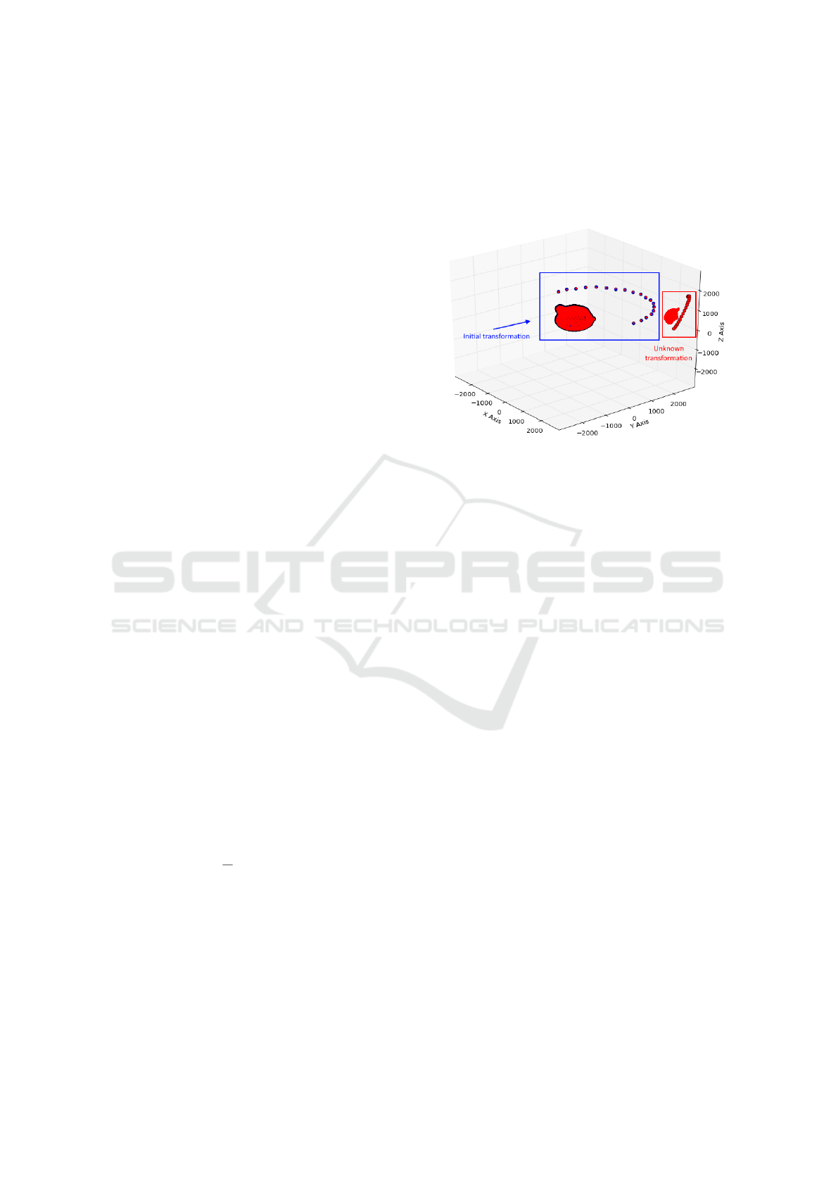
is seen in Figure 2, where the estimated transforma-

tion matrix is used on the Utah teapot, to transform it

to the coordinate’s initial position, together with the

unknown positions.

Figure 2: Visualization of the output of the least-squares

transformation estimation algorithm. The initial position,

orientation and scale are ﬁrst transformed to ”unknown”

ones. The estimation algorithm is then used to ﬁnd the

transformation from the ”unknown” one to the initial one.

The Utah teapot is added for easier visualization.

In the real world this is not the case, as measuring

equipment is always a subject to additive noise. This

needs to be taken into consideration, when using the

least-squares estimation algorithm. This will trans-

form Equation 3, where C = A + N, with A being the

known locations and N = [n

, n

, ...n

] is the added

noise component, with each noise n

= [n

, n

]

The next subsections will verify the sensor readings

and model the noise.

2.3 Verifying Sensor Readings

For the paper the sensor provided by DJI (DJI, 2017)

is used, as it has a very small margin of uncertainty in

the positioning information - less than 0.02m in ho-

rizontal direction and 0.03m vertically, in good we-

ather conditions. This precision needs to be veriﬁed,

before using it. Because the sensor works only when

attached to a drone controller, the whole platform is

used for the test. The sensor is started and its rea-

dings are saved each second for a period of 5 minu-

tes. The readings are taken when the whole platform

is on the ground, to eliminate inconsistencies from the

readings when the platform is in motion. The sen-

sor is then manually moved to another location and

the readings are again taken. The calculated position

standard deviation for the ﬁrst point is 0.0175m in ho-

rizontal direction and 0.0244m in height and for the

second point the standard deviations are 0.0174m and

VISAPP 2019 - 14th International Conference on Computer Vision Theory and Applications

886

0.0251m respectively. The values are thus in the inter-

val given in the documentation by DJI. With the real

world positioning uncertainty veriﬁed, the next step

is to create a number of synthetic testing scenarios,

where the uncertainty is used as a noise component.

These scenarios are used to investigate aspects of how

the GPS-RTK noise inﬂuences scale noise.

2.4 Synthetic Testing Scenarios

For the synthetic tests to be as close to a real world

test, the point sets are setup as real SfM capturing

positions. The tests are designed to determine the

amount of camera positions needed and the amount

of vertical camera bands. To gather enough variation

in the calculated scale after the noise input in each of

the tests, the least-squares estimation step is done a

number of times, each time with a different sampling

of noise input.

2.4.1 Number and Sampling of Image Positions

The ﬁrst synthetic test scenario looks at how the num-

ber of input camera positions affects the results of

the scale factor. The least-squares estimation method

requires at least two positions for estimation of the

transformation. In the paper by (Nikolov and Mad-

sen, 2016), a circular pattern of images is used, with

the position of each image, changing by 20 degrees.

This gave 18 images per circular pattern. For a sim-

pler and easier image capture for the real world test

scenarios described in the later sections, the circular

pattern is changed to a semi-circular one, leaving the

number of image positions to 18 again, giving a 10

degree separation between them. This gives the ﬁ-

nal testing interval - 3 to 18 positions. The minimum

number of positions is set to 3, as at least 3 points are

needed to estimate the 3D transformation. To test this

we start with the full number of 18 positions going

from 0 to 180 degrees. Then every time we lower the

number of positions we do not just remove the last

one, but we resample the left ones so they always co-

ver the whole interval of 0 to 180 degrees, but have

larger distance between them.

The synthetic test is done once without resam-

pling, starting with 18 positions and removing posi-

tions, until only the ﬁrst two are left. The second run

of the test is done with removing and resampling the

positions until only the 0 and 180 degree ones are left.

To model the positioning noise for each instance,

a random sampling of the uncertainty values captured

directly from the GPS-RTK. This of course introduces

the problem that not enough data has been captured

for a more diverse modeling of the uncertainty. We

will address this in the next subsection.

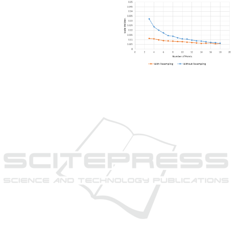
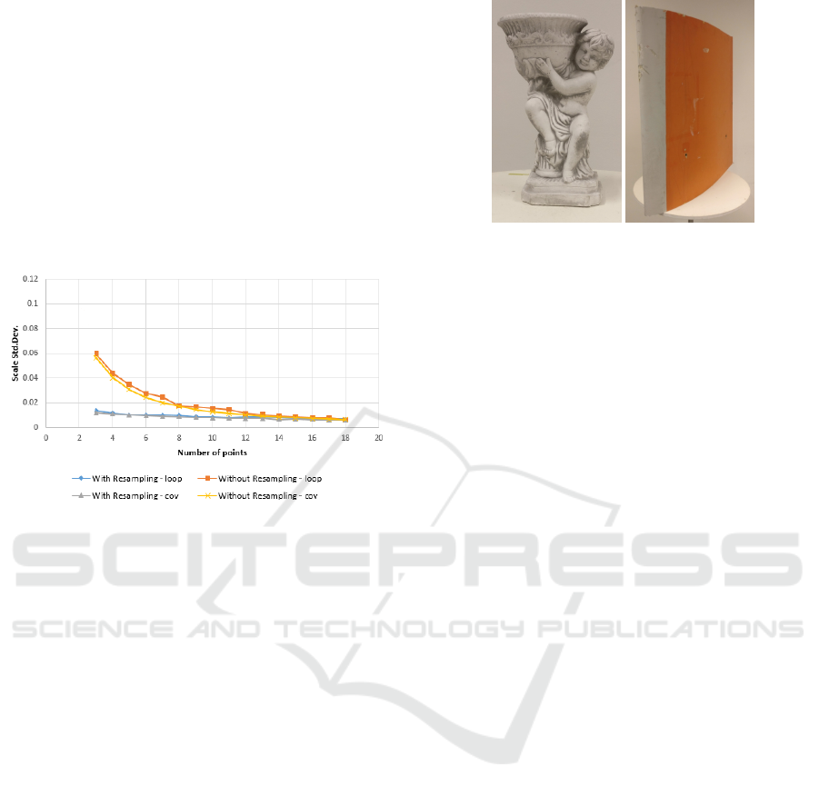
Figure 3: Results from the resampling versus no resampling

synthetic test. Resampling the captured positions so the ﬁrst

and last one are always at 0 and 180 degrees, after removing

positioning information drastically lowers the standard de-

viation of the calculated scale.

The obtained results are shown in Figure 3. When

resampling the positions, as points are removed the

additional separation between points helps with lo-

wering the calculated scale’s error. This is especially

evident up until 10 image positions. After that the

two methods have comparable result standard devi-

ations, which converge at 16 image positions. This

shows that if not all image positions can be captured,

it is better that the captured ones have maximum se-

paration. In addition, the standard deviation settles at

around 12 or 13 image positions.

2.4.2 Number of Vertical Bands

The second test scenario is designed to check how

many vertical bands of images and image positions

are needed. The previous test showed that worse scale

uncertainty is achieved when no resampling of the

points is present. This test will explore if better scale

uncertainty can be achieved with more vertical sepa-

ration between the positions, if no resampling is used.

The work of (Nikolov and Madsen, 2016), shows that

three bands of photos give the best possible recon-

struction results. The paper however manually sca-

les the output meshes, so no conclusions are given on

how the scaling is affected by the bands. To test this

we choose to test with one, two and three position

bands respectively. This will determine if the additi-

onal spatial change between the positions in different

bands, given to the least-squares estimator, will make

a difference to the calculated scale factor.

The synthetic test is started with one band of ver-

tical separation and 18 camera positions. The number

of positions is reduced by one for each test until only

3 positions are left. The same is done for two and

three vertical band tests. The estimated scale factor

is calculated from each and standard deviation is cal-

culated from all the possible results. The results are

Performance Characterization of Absolute Scale Computation for 3D Structure from Motion Reconstruction

887

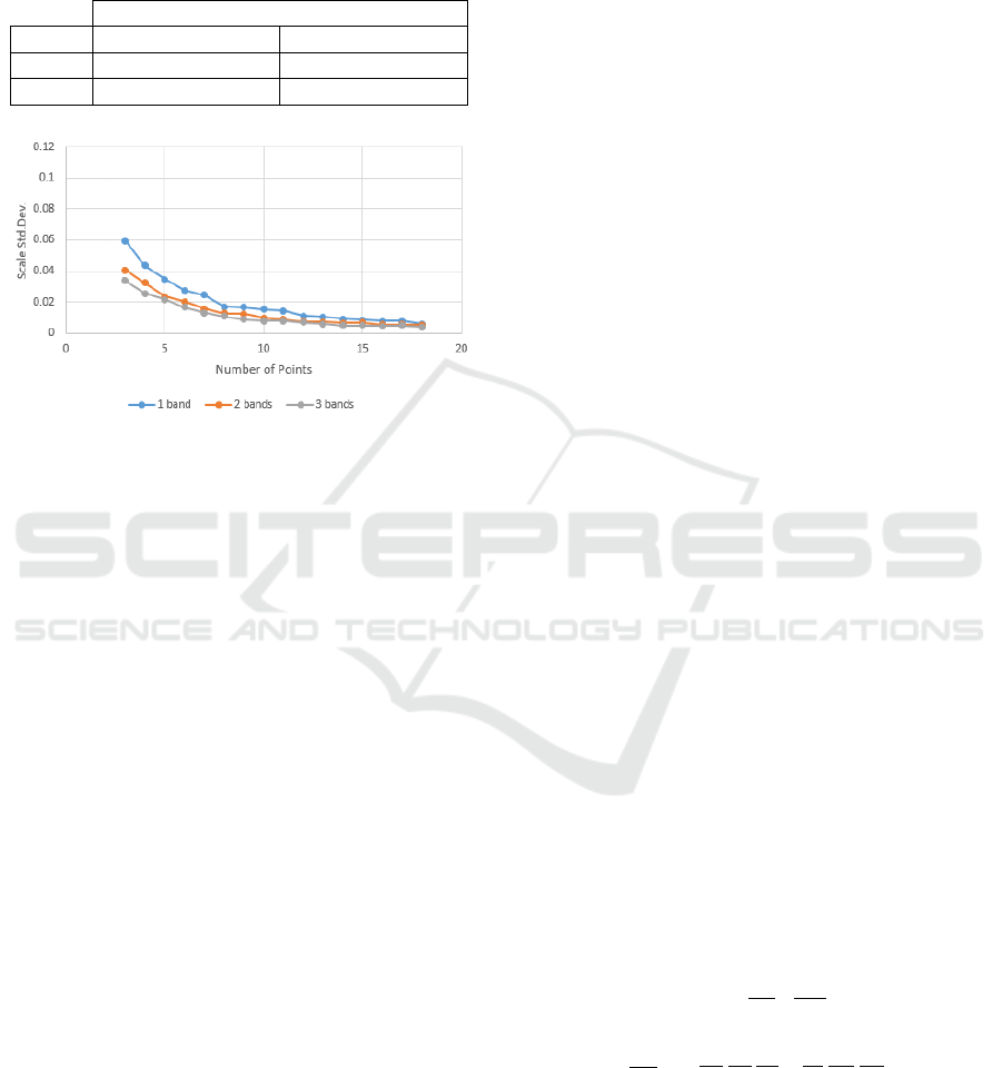
Table 1: Change in the scale standard deviation when going

from 1 to 2 bands and from 2 to 3 bands for the minimum

and maximum number of tested point positions. The change

from 2 to 3 bands is almost twice as small showing that the

gained accuracy, is not enough to offset the larger amount

of data, longer capturing time, etc.

Difference

Points 1 and 2 bands (%) 2 and 3 bands (%)

2 43.75 14.60

18 11.26 27.51

Figure 4: Results from capturing of positioning data from

different number of vertical bands. More vertical bands help

with the uncertainty of the scale. Both the larger number of

points and the additional spatial information help with that.

given in Figure 4.

As expected, the high standard deviation decre-

ases as we introduce additional vertical positions in

the form of more bands. This is both because of the

larger number of points and additional vertical sepa-

ration. If we look at the difference between the stan-

dard deviations of the calculated average scale we can

see a relation between the number of bands and num-

ber of points. The data is given in Table 1. When

more points are present in each band the gains won

by going from one to two bands are not big, but if

multiple bands need to be taken, then it will be much

better to capture three. When less points are present

in each band it is necessary to have as much bands

as possible, so the beneﬁts from the additional num-

ber of points and separation can be felt. To strike a

balance between number of bands captured and scale

precision gains, we choose to use two bands for the

real world testing scenario for testing against the state

of the art.

2.5 Covariance Propagating of

Positioning Noise

The way the noise is introduced in these synthetic

tests and the performance characterization of the scale

calculation is found, can be cumbersome, as the test

needs to be done a large number of times. A better

solution to this is using covariance propagation (Ha-

ralick, 2000) of the noise. This will give the relation

between the uncertainty in each GPS-RTK position

and the uncertainty in the ﬁnal calculated scale. The

idea has been shown to give good results (Madsen,

1997), as long as there are independent input parame-

ters, which are used in a function - no matter analyti-

cally or iteratively found, to calculate a set of output

parameters. As each captured GPS-RTK position is

used in the calculation of the scale factor through the

least-square estimation, this means that we can ex-

press the transformation calculation as represented as

s = f (C), where s is the estimated scale and C is the

GPS-RTK positioning set together with the introdu-

ced noise. We do not use the second positioning set B

obtained from the SfM reconstruction, as an input pa-

rameter, as it is treated as a constant. We use the met-

hod demonstrated in (Madsen, 1997), for determining

the covariance matrix of the input parameters. This of

course need to be done for each of the three dimensi-

ons for each of the points. The standard deviation of

the calculated scale will depend both on the standard

deviation of the uncertainty of the measured GPS-

RTK positions and the ﬁrst derivative of the function.

To ﬁnd the standard deviation of the scale, the ﬁrst or-

der approximation needs to be done to the covariance

matrix, as seen in Equation 4 and then used together

with the dependence of the scale to the positions in

all 3 dimensions, as given in Equation 5. Where ∆ is

the covariance matrix of Q and is described as Equa-

tion 6, for each of its dimensions. Thus Q is a com-

bined vector containing all the dimensional data for

each position Q = [x

, y

, z

, ..., x

, y

, z

]

1x3m

∆ =







0 0 . . . 0

0 σ

0 . . . 0

0 0 σ

. . . 0

. . . . . . . . . . . . . . . . . . . . . . . . .

0 . . . σ

0 0

0 . . . 0 σ

0 . . . 0 0 σ







3m×3m

(4)

∂s

∂Q

∆

∂s

∂Q

(5)

∂s

∂Q

∂s

∂x

∂s

∂y

∂s

∂z

...

∂s

∂x

∂s

∂y

∂s

∂z

(6)

To test if the iterative approach and the covari-

ance propagation approach will yield the same re-

sults. Again the testing scenario of subsection 2.4.1

is used, both with and without resampled positioning

data. The results can be seen in Figure 5. The two

approaches achieve closely matched results for both

VISAPP 2019 - 14th International Conference on Computer Vision Theory and Applications

888

positioning data types. The average difference bet-

ween the calculated scale standard deviation from 3

to 18 points between the two approaches, without res-

ampling positioning data is 12.07%, while with res-

ampling the difference falls to 4.88%. In addition the

covariance propagation approach follows a smoother

overall curve of progression, meaning less chance for

random noise in the estimated scale standard devia-

tion. This also demonstrates that the covariance pro-

pagation method gives very accurate estimation of the

standard deviation of the scale, while bypassing the

assumptions about the nature of the uncertainty’s dis-

tribution.

Figure 5: Comparing the interations approach to the covari-

ance propagation approach for calculating scale uncertainty

from position uncertainty. The comparison is made for dif-

ferent number of input positions and a different way of res-

ampling the positions.

3 REAL WORLD TESTING

Two objects are chosen for the test. They can be seen

in Figure 6. The objects are chosen because they re-

present two different 3D reconstruction use cases - the

statue represents a digital heritage use case, while the

wind turbine blade represents an industrial use case.

Both cases require precise scale estimation.

For each of the two objects, two vertical bands of

18 images are taken in a semi-circle. The horizontal

separation between the images is 10 degrees, while

the vertical separation between bands is 20 degrees.

The images are taken with a Canon 5Ds at maxi-

mum resolution 8688x5792. This camera is chosen,

so enough information is captured from the objects

and the chance of the 3D reconstruction failing or ha-

ving errors is minimized.

The camera positions are manually determined

with a laser range ﬁnder. This is done so that any

possible random positioning accuracy ﬂuctuations on

the GPS-RTK, caused by weather conditions, pres-

sure changes or environment effects are removed. A

second reason for this is that this way the experiment

(a) Angel Statue (b) Blade Segment

Figure 6: Two test objects used for 3D reconstruction.

Each represent different reconstruction challenges and re-

construction cases.

can be done in an indoor environment, removing the

possible illumination changes that can affect the ﬁnal

reconstruction.

For the reconstruction both PhotoScan and Con-

textCapture software is used. The two solutions have

a number of built-in ways to scale a model - using

point markers that the user directly adds to the model

and have been measured beforehand, printing marker

trackers and putting them around the scanned object

and detecting them in the images, adding coordina-

tes to the camera positions from GPS. For testing our

proposed solution, we have chosen the method that

is most relevant - adding camera positions, together

with the images and using them to scale the object.

Because the built-in solutions do not have a mea-

surement of the uncertainty of the scaling, the compa-

rison will be done only on the basis of the calculated

scaling factors. For comparing the calculated scale

factors, the reconstructed objects will be scaled using

these factors and the distance will be measured ma-

nually on the real world object and the scaled recon-

struction.

As there are no ground truth scaled model to com-

pare the scales from the three methods, a manual me-

asuring of the objects is chosen. A number of parts of

the two real world objects are measured with a caliper,

which has a resolution of ±0.02mm, when measuring

objects below 100mm. The reconstructed and scaled

model are imported into CloudCompare (Girardeau-

Montaut, 2003) for measuring the same parts. By

measuring multiple parts of the models and averaging

the difference between the real world measurement

and the scaled model measurement, the effects of the

possible human errors, while manually measuring are

minimized.

The obtained scaled models are given in Figure 6.

Just by looking at the models, no observable diffe-

rence can be seen. Table 2 contains the average me-

Performance Characterization of Absolute Scale Computation for 3D Structure from Motion Reconstruction

889

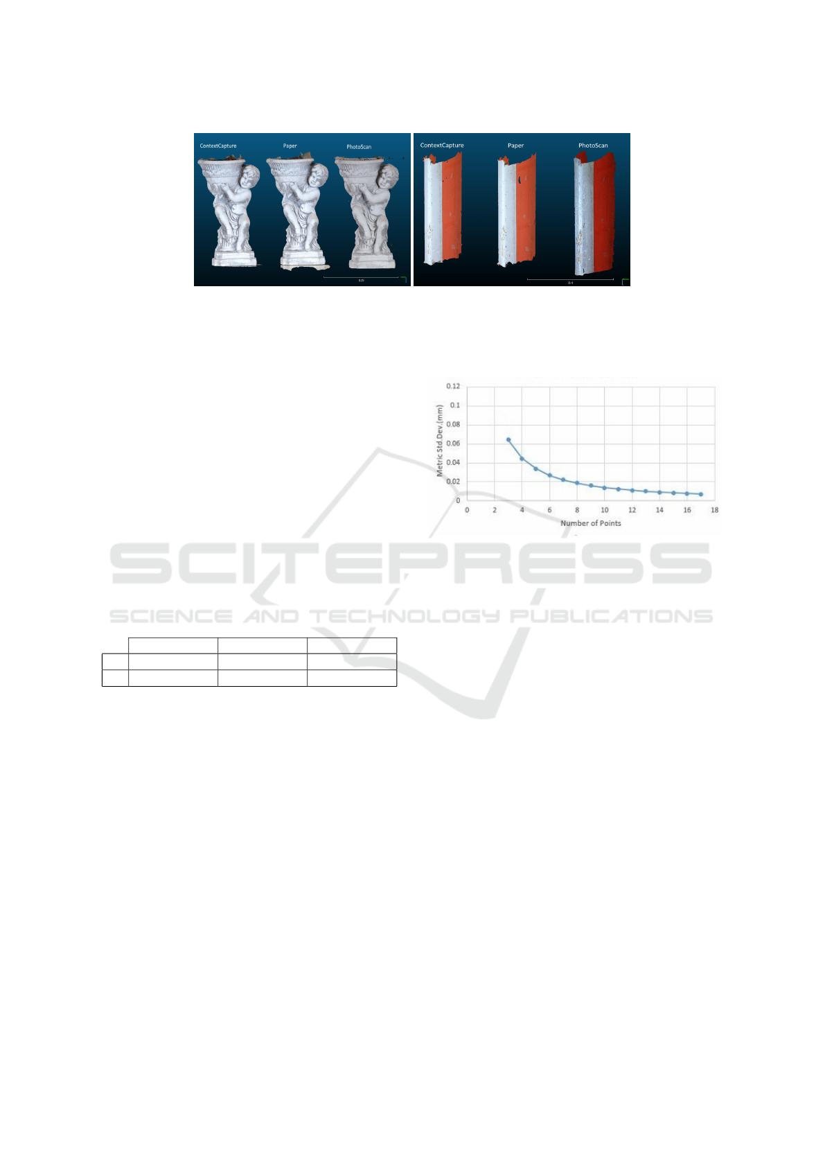
(a) Angel Statue (b) Blade Segment

Figure 7: Reconstructed and scaled model. The ContextCapture and PhotoScan reconstructions are scaled using the built-in

solutions in the software. For our proposed solution(Paper), the unscaled ContextCapture reconstruction is used as basis. The

brightness difference in the models is due to the different ways the programs normalize the texture color. In addition the

model from PhotoScan reconstructed a larger portion of the blade and looks larger even though the scale is comparable.

asured distance errors from measuring ten different

parts in the real world and on the reconstructed ob-

jects, as well as the standard deviation from the mea-

surements. The results show that our proposed solu-

tion gives better results, because the mean error dis-

tance is the lowest compared to the other. Even if

we factor in the manual repeated measurement error,

shown as the standard deviation of the distance in the

table, the results obtained by our method are better or

the same as the build in solutions.

Table 2: Average distance error between measurements

from the real world object and the reconstructed model, for

the two tested objects - angel (A) and blade (B). The results

are in mm and the comparison is made between our pro-

posed solution (Paper) and the built-in scaling solutions in

ContextCapture (CC) and PhotoScan (PS).

Paper (mm) CC (mm) PS (mm)

A 0.35 ± 0.063 0.48 ± 0.069 1.04 ± 0.093

B 0.18 ± 0.012 0.23± 0.008 0.56 ± 0.009

metric

= D

S f M

· σ

(7)

Furthermore the scale uncertainty in mm can be

also easily measured through our proposed solution.

We can take two random points from the unscaled

measured object and calculate the Euclidean distance

between them in unknown units - D

S f M

. As we have

calculated the scale uncertainty, denoted as σ

, we can

use Equation 7 as given in the book by (DeGroot and

Schervish, 2012), to calculate scaled distance uncer-

tainty σ

metric

in the chosen metric. To demonstrate

how this uncertainty can be useful, we recalculate the

real world reconstruction’s scale uncertainty, by using

different number of position data - from 2 to 18. Each

uncertainty is then used to ﬁnd the metric uncertainty

of the distance between the same two randomly cho-

sen points. The results from the test can be seen in

Figure 8. The calculated metric uncertainty decreases

with the introduction of more and more point positi-

ons.

Figure 8: Correlation between the number of positions used

to calculate the scale uncertainty and the metric uncertainty

when measuring the real world distance between two points

on a object.

4 CONCLUSION AND FUTURE

WORK

In our paper we presented a pipeline for computing

the absolute scale of a 3D model reconstructed using

SfM. Our method relies on using external positioning

information from a GPS-RTK sensor, which has an

inherent uncertainty present in the provided data. We

provide an analysis of this uncertainty and how it pro-

pagates to the calculated absolute scale and results in

a scale uncertainty. Through a series of tests we de-

monstrated how changes to the number of positions

used and their spatial relationship can also inﬂuence

the scale uncertainty. We tested two ways to ﬁnd the

scale uncertainty - an iterative method and a mathe-

matical covariance propagation of noise method.

Finally, we tested our proposed pipeline against

the scaling solutions available in state of the art SfM

software solutions - ContextCapture and PhotoScan.

We demonstrate that we achieve better results, on top

of providing more information about the scaling un-

certainty.

VISAPP 2019 - 14th International Conference on Computer Vision Theory and Applications

890

As a extension to the current paper, we propose

testing the pipeline using data captured through drone

ﬂights. This way the GPS-RTK positioning informa-

tion can be tested in different weather and environ-

ment conditions. Additionally the testing on objects

with different sizes will provide data on how the met-

hod scales with size and if the uncertainty depends on

the size of the scanned object. Finally, different po-

sitioning systems would also be tested and modeled -

both indoor and outdoor, to make the pipeline more

versatile.

ACKNOWLEDGEMENTS

This work is funded by the LER project no. EUDP

2015-I under the Danish national EUDP programme.

This funding is gratefully acknowledged.

REFERENCES

Agisoft (2010). Agisoft: Photoscan. http://www.agisoft.

com/. Accessed: 2018-09-06.

Bay, H., Tuytelaars, T., and Van Gool, L. (2006). Surf:

Speeded up robust features. In European conference

on computer vision, pages 404–417. Springer.

Bentley (2016). Bentley: Contextcapture. https://www.

bentley.com/. Accessed: 2018-09-06.

CapturingReality (2016). Capturingreality: Reality capture.

https://www.capturingreality.com/. Accessed: 2018-

09-06.

Corti, A., Giancola, S., Mainetti, G., and Sala, R. (2016).

A metrological characterization of the kinect v2 time-

of-ﬂight camera. Robotics and Autonomous Systems,

75:584–594.

Daakir, M., Pierrot-Deseilligny, M., Bosser, P., Pichard, F.,

Thom, C., and Rabot, Y. (2016). Study of lever-arm

effect using embedded photogrammetry and on-board

gps receiver on uav for metrological mapping purpose

and proposal of a free ground measurements calibra-

tion procedure. ISPRS Annals of Photogrammetry, Re-

mote Sensing & Spatial Information Sciences.

DeGroot, M. H. and Schervish, M. J. (2012). Probability

and statistics. Pearson Education.

DJI (2017). D-rtk gnss. https://www.dji.com/. Accessed:

2018-09-06.

Dugan, M. (2018). Rtk enhanced precision geospatial lo-

calization mechanism for outdoor sfm photometry ap-

plications. Robotics Research Journal.

Girardeau-Montaut, D. (2003). Cloudcompare. http://www.

cloudcompare.org/. Accessed: 2018-09-12.

Haralick, R. M. (2000). Propagating covariance in compu-

ter vision. In Performance Characterization in Com-

puter Vision, pages 95–114. Springer.

Jamaluddin, A., Mazhar, O., Jiang, C., Seulin, R., Morel,

O., and Foﬁ, D. (2017). An omni-rgb+ d camera rig

calibration and fusion using uniﬁed camera model for

3d reconstruction. In 13th International Conference

on Quality Control by Artiﬁcial Vision 2017, volume

10338.

Lowe, D. G. (2004). Distinctive image features from scale-

invariant keypoints. International journal of computer

vision, 60(2):91–110.

Madsen, C. B. (1997). A comparative study of the robust-

ness of two pose estimation techniques. Machine Vi-

sion and Applications, 9(5-6):291–303.

Nikolov, I. and Madsen, C. (2016). Benchmarking close-

range structure from motion 3d reconstruction soft-

ware under varying capturing conditions. In Euro-

Mediterranean Conference, pages 15–26. Springer.

Rabah, M., Basiouny, M., Ghanem, E., and Elhadary, A.

(2018). Using rtk and vrs in direct geo-referencing of

the uav imagery. NRIAG Journal of Astronomy and

Geophysics.

Sarbolandi, H., Leﬂoch, D., and Kolb, A. (2015). Kinect

range sensing: Structured-light versus time-of-ﬂight

kinect. Computer vision and image understanding,

139:1–20.

Sarker, M., Ali, T., Abdelfatah, A., Yehia, S., and Elaksher,

A. (2017). a cost-effective method for crack detection

and measurement on concrete surface. The Internatio-

nal Archives of Photogrammetry, Remote Sensing and

Spatial Information Sciences, 42:237.

Schonberger, J. L. (2016). Colmap. https://colmap.github.

io. Accessed: 2018-09-06.

Sch

oning, J. and Heidemann, G. (2016). Taxonomy of 3d

sensors. Argos, 3:P100.

Sch

ops, T., Sattler, T., H

ane, C., and Pollefeys, M. (2015).

3d modeling on the go: Interactive 3d reconstruction

of large-scale scenes on mobile devices. In 3D Vision

(3DV), 2015 International Conference on, pages 291–

299. IEEE.

Triggs, B., McLauchlan, P. F., Hartley, R. I., and Fitzgibbon,

A. W. (1999). Bundle adjustmenta modern synthesis.

In International workshop on vision algorithms, pages

298–372. Springer.

Umeyama, S. (1991). Least-squares estimation of transfor-

mation parameters between two point patterns. IEEE

Transactions on Pattern Analysis & Machine Intelli-

gence, (4):376–380.

VisualSFM, C. W. (2011). A visual structure from motion

system.

Performance Characterization of Absolute Scale Computation for 3D Structure from Motion Reconstruction

891