Decomposing Constraint Satisfaction Problems by Means of Meta
Constraint Satisfaction Optimization Problems
Sven L
¨
offler, Ke Liu
a
and Petra Hofstedt
Brandenburg University of Technology Cottbus-Senftenberg, Germany
Department of Mathematics and Computer Science, MINT, Germany
Programming Languages and Compiler Construction Group, Konrad-Wachsmann-Allee 5, 03044 Cottbus, Germany
Keywords:
Constraint Programming, CSP, CSOP, Decomposition, Parallelization, Optimization, Parallel Constraint
Solving, Problem Splitting.
Abstract:
This paper describes a new approach to decompose constraint satisfaction problems (CSPs) using an auxiliary
constraint satisfaction optimization problem (CSOP) that detects sub-CSPs which share only few common
variables. The purpose of this approach is to find sub-CSPs which can be solved in parallel and combined
to a complete solution of the original CSP. Therefore, our decomposition approach has two goals: 1. to
evenly balance the workload distribution over all cores and solve the partial CSPs as fast as possible and 2. to
minimize the number of shared variables to make the join process of the solutions as fast as possible.
1 INTRODUCTION
Constraint programming (CP) is a powerful method
to model and solve (not only but especially) NP-
complete problems in a declarative way. Typical re-
search problems in CP are rostering, graph coloring,
optimization, and satisfiability (SAT) problems (Mar-
riott, 1998).
Since the search space of CSPs is very big and
the solution process often needs an extremely high
amount of time we are always interested in improve-
ment and optimization of the solution process. Paral-
lel constraint solving is a promising way to enhance
the performance of constraint programming. The
four most common kinds of parallel constraint pro-
gramming are parallel search (Hamadi, 2002; Nguyen
and Deville, 1998), parallel consistency (R
´
egin et al.,
2013; Rolf and Kuchcinski, 2009), combining parallel
search and parallel consistency (Rolf and Kuchcinski,
2009) and distributed CSPs (Faltings, 2006; Yokoo
and Hirayama, 2000). Parallel search can furthermore
be divided by the way of portfolios, problem splitting,
and search space splitting (e. g. embarrassingly par-
allel search (R
´
egin et al., 2013)).
The presented approach finds decompositions of
CSPs in a way that each part has approximately the
same size (number of variables) and as little as possi-
a
https://orcid.org/0000-0002-5256-9253
ble shared variables so that we can use it effectively
for problem splitting. Because the algorithm not only
distributes the variables but also the constraints of the
CSP it also can be used for parallel consistency tech-
niques.
2 PRELIMINARIES
In this section, we introduce the necessary definitions,
methods and theoretical considerations which are
the basis of our approach. We consider constraint
satisfaction problems (CSPs), constraint satisfaction
optimization problems (CSOP) and sub-CSPs which
are defined as follows.
CSP (Dechter, 2003) A constraint satisfaction prob-
lem (CSP) is defined as a 3-tuple P = (X,D,C)
with X = {x
1
,x
2
,...,x
n
} is a set of variables,
D = {D
1
,D
2
,..., D
n
} is a set of finite domains where
D
i
is the domain of x
i
and C = {c
1
,c
2
,...,c
m
} is a set
of primitive or global constraints containing between
one and all variables in X.
Sub-CSP Let P = (X,D,C) be a CSP. For C
0
⊆
C we define P
sub
= (X
0
,D
0
,C
0
) such that X
0
=
S
c∈C
0
scope(c), where scope(c) gives the variables
in a constraint c (see below) with corresponding do-
mains D
0
= {D
i
| x
i
∈ X
0
} ⊆ D.
Löffler, S., Liu, K. and Hofstedt, P.
Decomposing Constraint Satisfaction Problems by Means of Meta Constraint Satisfaction Optimization Problems.
DOI: 10.5220/0007455907550761
In Proceedings of the 11th International Conference on Agents and Artificial Intelligence (ICAART 2019), pages 755-761
ISBN: 978-989-758-350-6
Copyright
c
 2019 by SCITEPRESS – Science and Technology Publications, Lda. All rights reserved
755

CSOP (Rossi et al., 2006; Tsang, 1993) A constraint
satisfaction optimization problem (CSOP) P
opt
=
(X, D,C, f ) is defined as a CSP with an optimiza-
tion function f that maps each solution to a numerical
value.
2.1 Definitions and Methods
In this section we define methods required by our
algorithm. Let a CSP P = (X, D,C) be given.
scope(c) (Dechter, 2003) The method scope has a
constraint c ∈ C as input and returns all variables
X
0
⊆ X which are covered by this constraint.
cons(x) The method cons has a variable x ∈ X as
input and returns the set of constraints C
0
⊆ C which
cover variable x.
sharedVars(c
1
,c
2
) We define a variable x ∈ X which
is covered by two constraints c
1
and c
2
∈ C as shared
variable of c
1
and c
2
. Based on this, the method
sharedVars gets two constraints c
1
and c
2
as input and
returns all shared variables of the constraints. Analo-
gously if sharedVars gets two sub-CSPs P
1
and P
2
as
input it returns the shared variables of the sub-CSPs.
2.2 Problem Splitting
The problem splitting process has three steps.
1. Decompose the given CSP P = (X,D,C) in k sub-
CSPs P
sub
= {P
1
,...,P
k
} in a way that each sub-
CSP P
i
= (X
i
,D
i
,C
i
)∀i ∈ 1,. . . ,k has a subset of
constraints C
i
⊆ C, where C
i
∩C
j
=
/
0 ∀i, j,i 6= j
and
S
k
i=1
C
i
= C. Note that the constraints of
the CSPs P
i
are disjoint but the variables can be
shared.
2. Solve all sub-CSPs in P
sub
.
3. Join the results of the sub-CSPs in P
sub
to a solu-
tion of the original CSP P.
The time complexity of problem splitting depends
essentially on two considerations. First, the time
needed for solving the most complex sub-CSP P
i
, be-
cause the algorithm can only continue if all sub-CSPs
were solved. If D
max
is the biggest domain of vari-
ables in X then the complexity for finding all solutions
of sub-CSP P
i
is in O(|D
max
|
|X
i
|
).
The second influence on the overall effort for
problem splitting comes from the time needed to join
the solutions of the sub-CSPs P
i
and P
j
. Algorithms
like sort-merge join can join two tables S and R in
O(N log N), where N is the maximum of |S| and
|R|. In our case S and R are the partial solutions
of the shared variables of the sub-CSPs P
i
and P
j
.
So let n
SV
be the number of shared variables n
SV
=
|sharedVars(P
i
,P
j
)|. This means that the maximum
number of different value assignments for the shared
variables (and so the maximum size N of S and R)
must be smaler or equal |D
max
|
n
SV
. That leads to a
time complexity for merging two sub-CSPs P
i
and P
j
given by (1).
O(|D
max
|
n
SV
log(|D
max
|
n
SV
)) (1)
So the overall complexity for both points is given by
(2) .
O(|D
max
|
max(|X
i
|,|X
j
|)
+|D
max
|
n
SV
log(|D
max
|
n
SV
)) (2)
If more than two sub-CSPs P = {P
1
,...,P
k
|k > 2}
are created then we can join them step after step like
a binary tree. In each step we join two sub-CSPs.
In the next step two of the before joined sub-CSPs
will be joined and so on. Let n
maxSV
be the maxi-
mum number of shared variables of all join processes.
The complexity for the biggest join process is then in
O(|D
max
|
n
maxSV
log(|D
max
|
n
maxSV
)).
So the time complexity of the problem splitting
process depends on the size of the maximal sub-CSP
P
i
∈ {P
1
,...,P
k
} and the maximum number of shared
variables in all join processes. Thus, our decomposi-
tion CSOP will minimize one or both of these values.
3 THE META CSOP FOR THE
DECOMPOSITION OF CSPS
In this section, we present an approach to decompose
CSPs into sub-CSPs using a Meta CSOP.
3.1 A CSOP for Separating a CSP into
Sub-CSPs
For detecting k sub-CSPs {P
1
,...,P
k
} of a given
CSP P = (X,D,C) where X = {x
1
,...,x
n
},
D = {D
1
,...,D
n
} and C = {C
1
,...,C
m
} we
define a CSOP P
opt
= (X
0
,D
0
,C
0
, f ) where
X
0
= {x
0
j
|∀ j ∈ {1, ...,m}} ∪ {x
opt
}, D
0
= {D
0
j
=
{1,...,k}|∀ j ∈ {1, ...,m}} ∪ {D
opt
= {0,..., ∞}},
C
0
= {cspSplit(X
0
,M, k, x
opt
,w) ∪ {count(l,X
0
,≥
1)|∀l ∈ {1,...,k}}, and f = minimize(x
opt
) which
finds an optimized decomposition of P into k
sub-CSPs P
1
,...,P
k
if they exist.
For each constraint c
j
∈ C a variable x
j
with do-
main D
0
j
= {1, . . . , k} is created. The value assign-
ment v for a variable x
j
represents that the correspond-
ing constraint c
j
is part of sub-CSP P
v
. The count
constraint is defined like in (Prud’homme et al., 2017)
ICAART 2019 - 11th International Conference on Agents and Artificial Intelligence
756

and ensures that no empty sub-CSP is created. More
accurate, the count(l,X
0
,≥ 1) constraint guarantees
that the value l occur at least one time (≥ 1) in the
variable set X
0
. The cspSplit constraint is explained
in detail in the next section. The variable x
opt
is used
to optimize the sizes of the sub-CSPs (P
1
,...,P
k
) and
the shared variables between them, as these are the
main factors which influence the problem splitting
complexity (explained above, see 2.2). The objective
function f minimizes the x
opt
variable with domain
D
opt
= {1,...,∞} which is also explained in the fol-
lowing section.
3.2 The cspSplit Constraint
We developed a new constraint, cspSplit, which par-
titionate constraints of a given CSP P into a set of
sub-CSPs {P
1
,...,P
k
}.
Doing this the cspSplit constraint takes a set of
variables X
0
, a two dimensional array of integers M,
the number of sub-CSPs k, the optimization vari-
able x
opt
and a two dimensional weight vector w =
(w
1
,w
2
) as input.
Each variable x
j
∈ X
0
represents the correspond-
ing constraint c
j
∈ C of the given CSP P. If the vari-
able x
j
is set to a value v it means that the constraint
c
j
is part of the sub-CSP P
v
and therefore not included
in other sub-CSPs.
The two dimensional array M indicates which
variables are covered by which constraints. For each
constraint c
j
∈ C of CSP P exists one line which con-
tains all variables X
c
which are covered by the con-
straint (X
c
= {x
i
|x
i
∈ scope(c)}). So the entry M
j,l
= i
follows from the fact that constraint c
j
contains vari-
able x
i
at l-th position.
Algorithm 1 shows the propagation algorithm of
the cspSplit constraint. In line 1, a binary vector of
size |X| (number of variables in the original CSP P)
will be created for all k sub-CSPs which should be
created. So b
1
represents the first sub-CSP and b
k
the
last. For each vector b
l
the i-th entry (∀i ∈ {1,...,|X|})
represents that the i-th variable x
i
∈ X of CSP P is part
of the sub-CSP P
l
. Each vector is instantiated with
values null so no variable is associated to a sub-CSP
at the beginning.
In lines 2 to 6, the variables x
i
∈ X
0
(representation
of c
i
in the original CSP P) are checked whether they
are already instantiated. If a variable x
i
is instantiated
to value v then this means that constraint c
i
∈ C of P is
part of the sub-CSP P
v
. If such assignments exist, then
the algorithm sets all bits in b
v
to true which represent
variables that are covered by the constraint c
i
(line 5
and 6).
Algorithm 1: The cspSplit algorithm.
Data: variables X
0
, int × int M, int k,
variable X
opt
, intVector w = (w
1
,w
2
)
1 Create k binary vectors b
1
,. . . ,b
k
of size |X|
2 forall x
i
∈ X
0
do
3 if (isInstantiated(x
i
)) then
4 int v = x
i
.getValue()
5 forall j ∈ {1,...,|scope(c
i
)|} do
6 b
v
[M
i, j
] = 1
7 forall x
i
∈ X
0
do
8 if (isNotInstantiated(x
i
)) then
9 forall j ∈ {1,...,k} do
10 if (∀b
j
[M
i,∗
] == 1) then
11 instantiate x
i
to j
12 continue with loop in line 7
13 int minValue = w
1
∗ maximum({number of
ones in b
i
|∀i ∈ {1,. . . , k}})+
w
2
∗ maximum(number of shared variables)
14 update lowerBound of x
opt
to minValue
In lines 7 to 11, constraints c
i
∈ C of P (repre-
sented by x
i
∈ X
0
of P
opt
) are checked if they are as-
signed to a sub-CSP. If a constraint c
i
has not yet been
assigned to a sub-CSP, then we check whether there is
a sub-CSP P
j
which contains all variables which are
covered by this constraint. If this is the case then the
constraint will be assigned to that sub-CSP (x
i
instan-
tiate to j).
In line 13, the new lower bound of the optimiza-
tion variable is calculated.
Finally, in line 14, the lower bound of the opti-
mization variable is updated.
Remarks: The steps in line 7-12 associate con-
straints to a sub-CSP for which no variables must be
added to this sub-CSP. This does not influence the cor-
rectness of the algorithm but it can increase the solu-
tion speed heuristically.
The minValue (in line 13) connects exactly the
detected parameters (Section 2.2) which has impact
on the solution speed of problem splitting multiplied
with a weight vector. The number of ones in b
i
is ex-
actly the number of variables in the sub-CSP P
i
. The
number of shared variables can be calculated by cre-
ating the intersection of two vectors b
i
and b
j
. The
weight vector allows the user to decide whether he/
she wants to improve the solution process or the join
process more.
Finding a perfect solution for the CSOP P
opt
is
also very time consuming and in this case may not
be useful. It is likely to find a good solution in a short
time.
Decomposing Constraint Satisfaction Problems by Means of Meta Constraint Satisfaction Optimization Problems
757

3.3 The Complexity of the CspSplit
Algorithm
In this section we consider the complexity of our csp-
Split algorithm. Creating k binary vectors of size
|X| = n has complexity O(k ∗ n) (line 1).
The cost in lines 2 to 6 depends only from the two
nested loops. The other cost are more or less constant.
So the complexity for this part of the algorithm (lines
2 to 6) is in O(m ∗ n
max
), where m is the number of
variables in X
0
of P
opt
(equal to the number of con-
straints in C of P), and n
max
is the maximum number
of variables a constraint c
i
in C of P has.
The cost in line 8, 11 and 12 are constant again
so it is only necessary to multiply the number of rep-
etitions of the two loops (m ∗ k) with the complexity
of the forall statement, which is in O(n
max
). So the
overall complexity of this part (lines 7 to 12) is in
O(m ∗ k ∗ n
max
).
The cost for the calculation of the minValue is in
O(n ∗ k +(k −1)∗ n
2
). The complexity of the calcula-
tion of the maximum number of shared variables re-
sults from the complexity of a join O(n∗n) multiplied
with the number of joins (k − 1) (k/2 joins on the first
level, then join the k/4 joined variable sets again and
so on).
This leads to an overall complexity of O(k ∗ n) +
(m∗n
max
)+(m ∗k ∗n
max
)+(n ∗k +(k − 1)∗n
2
)). Be-
cause of n
max
≤ n it is in O(m∗k ∗ n +k ∗ n
2
) where m
is the number of constraints in P, n is the number of
variables in P and k the number of sub-CSPs we want
to create.
4 EXAMPLES AND
EXPERIMENTAL RESULTS
In this section, we first present an example for the in-
puts and outputs of our Meta CSOP and then some
of our experimental results. We show that our Meta
CSOP can be used for the decompostion of big prob-
lems in an acceptable time. In the third part we give a
concrete example which improves the solution speed
of a CSP significantly by the use of the CSOP.
4.1 Example for the Meta CSOP
For the better understanding we show a small exam-
ple CSP P = (X,D,C), the corresponding Meta CSOP
and a result of its decomposition.
Consider a CSP P = (X,D,C) where X =
{x
1
,...,x
6
}, D = {D
1
= ... = D
6
= {1,2, 3,4, 5}}
and C = {c
1
= (x
1
> x
2
),c
2
= (x
2
< x
3
),c
3
= (x
4
>
x
5
),c
4
= (x
6
> x
5
),c
5
= (x
1
+ x
2
= x
3
),c
6
= (x
2
+
x
4
= x
5
+ x
6
),c
7
= (x
2
6= x
4
)}.
We follow the steps in Section 3.1 and want to
detect k = 2 sub-CSPs. This yields the Meta CSOP
P
opt
= (X
0
,D
0
,C
0
, f ) where X
0
= {x
0
1
,...,x
0
7
,x
opt
},
D = {D
0
1
,...,D
0
7
,D
opt
} with D
0
1
= ... = D
0
7
= {1, 2}
and D
opt
= {0,...,∞}, C
0
= {cspSplit({x
0
1
,...,x
0
7
},
M,2, x
opt
,w),count(1, {x
0
1
,...,x
0
7
}, ≥, 1), count(2,
{x
0
1
,...,x
0
7
},≥,1)} and f = minimize(x
opt
).
For the reason that the original CSP P has seven
constraints (|C| = 7), the Meta CSOP P
opt
has seven
variables (|X
0
| = 7) with domains {1, 2} (because
there will be two sub-CSPs, k = 2) and one opti-
mization variable x
opt
with domain {0,...,∞}. The
cspSplit constraint gets the variables x
0
1
,...,x
0
7
, the
matrix M (see in (3)) the number of sub-CSPs (k = 2),
the optimization variable x
opt
and a weight vector w
as input.
The matrix M indicates in each line i and row j if
variable x
j
∈ X is covered by constraint c
i
∈ C. The
weight vector w = (w
1
,w
2
) can be chosen freely, de-
pending on whether the user wants to prioritize a min-
imum number of variables per sub-CSP (increase w
1
)
or a minimum number of shared variables between
both sub-CSPs (increase w
2
).
M =
1 1 0 0 0 0
0 1 1 0 0 0
0 0 0 1 1 0
0 0 0 0 1 1
1 1 1 0 0 0
0 1 0 1 1 1
0 1 0 1 0 0
(3)
For weight vector w = (1, 1) the algorithm gener-
ates the following perfext solution x
0
1
= 1,x
0
2
= 1,x
0
3
=
2,x
0
4
= 2, x
0
5
= 1, x
0
6
= 2, x
0
7
= 2, x
opt
= 5. The value 5
for x
opt
results from the maximum number of vari-
ables in each sub-CSP (in this case the first sub-CSP
has three variables and the second four) plus the num-
ber of shared variables between both sub-CSPs (in
this case one because we have only the shared vari-
able x
2
).
The solution of the Meta CSOP P
opt
leads to the
following sub-CSPs P
1
and P
2
of the CSP P:
P
1
= (X
1
,D
1
,C
1
) where X
1
= {x
1
,x
2
,x
3
}, D
1
=
{D
1
,D
2
,D
3
} and C
1
= {c
1
= (x
1
> x
2
),c
2
= (x
2
<
x
3
),c
5
= (x
1
+ x
2
= x
3
)}.
P
2
= (X
2
,D
2
,C
2
) where X
2
= {x
2
,x
4
,x
5
,x
6
}, D
2
=
{D
2
,D
4
,D
5
,D
6
} and C
2
= {c
3
= (x
4
> x
5
),c
4
=
(x
6
> x
5
),c
6
= (x
2
+ x
4
= x
5
+ x
6
),c
7
= (x
2
6= x
4
)}.
ICAART 2019 - 11th International Conference on Agents and Artificial Intelligence
758

Table 1: Experimental results for the Meta CSOP of the benchmark suite from (Gottlob and Samer, 2009). (*Values after 1s,
10s and 10min).
4 sub-CSPs 8 sub-CSPs 16 sub-CSPs
Name (Cons, Vars) Max Vars* Shared Vars* Max Vars* Shared Vars* Max Vars* Shared Vars*
adder 99(496, 694) 279, 266, 239 259, 233, 188 160, 159, 141 312, 302, 220 85, 80, 77 347, 290, 275
NewSystem4(418, 718) 273, 260, 245 226, 214, 172 144, 142, 132 224, 222, 183 78, 77, 72 233, 246, 219
bridge 50(452, 452) 184, 178, 156 171, 180, 120 107, 105, 94 214, 206, 174 68, 61, 56 277, 263, 238
bridge 75(677, 677) 301, 264, 252 327, 241, 224 182, 151, 145 348, 300, 260 107, 106, 85 432, 417, 335
bridge 99(893, 893) 420, 349, 322 441, 343, 262 256, 210, 194 501, 418, 365 141, 123, 107 576, 492, 404
grid2D 30(450, 450) 212, 206, 167 235, 233, 143 136, 133, 115 295, 293, 230 91, 85, 72 348, 338, 286
grid2D 35(612, 613) 359, 271, 256 460, 268, 248 216, 180, 167 456, 388, 329 128, 115, 99 492, 473, 402
grid2D 40(800, 800) 462, 345, 315 430, 320, 278 286, 236, 216 533, 496, 473 169, 152, 127 679, 636, 550
grid2D 45(1013, 1013) 590, 456, 387 601, 336, 330 375, 305, 266 792, 622, 549 214, 200, 166 837, 791, 714
grid2D 50(1250, 1250) 735, 627, 446 817, 503, 364 468, 418, 320 1036, 729, 663 266, 258, 210 1056, 978, 875
grid2D 60(1800, 1800) 1047, 1013, 624 1314, 712, 447 718, 651, 475 1437, 1159, 963 419, 386, 301 1532, 1483, 1220
grid2D 70(2450, 2450) 1461, 1427, 876 1911, 1311, 626 954, 907, 673 2001, 1823, 1427 593, 526, 424 2066, 2059, 1719
grid2D 75(2812, 2813) 1667, 1655, 991 2100, 1563, 736 1092, 1058, 728 2297, 2215, 1521 696, 600, 491 2364, 2332, 1984
s713(412, 447) 182, 170, 159 165, 139, 132 101, 94, 91 187, 164, 145 57, 56, 51 203, 210, 178
s838(422, 457) 190, 183, 168 189, 171, 138 111, 106, 101 200, 198, 188 64, 63, 58 247, 227, 213
s953(424, 440) 193, 188, 178 213, 190, 169 115, 112, 106 224, 225, 202 66, 65, 61 248, 264, 240
s1196(547, 561) 239, 234, 223 239, 228, 205 145, 142, 136 279, 276, 267 84, 81, 79 312, 312, 300
s1238(526, 540) 236, 231, 221 237, 227, 204 143, 139, 134 269, 255, 265 84, 80, 78 308, 282, 280
s1423(731, 748) 316, 286, 274 290, 249, 210 185, 175, 165 356, 320, 290 108, 100, 97 426, 361, 353
s1488(659, 667) 264, 254, 247 211, 212, 185 158, 152, 149 272, 245, 239 96, 91, 89 329, 329, 315
s1494(653, 661) 267, 254, 242 244, 218, 185 159, 154, 146 279, 267, 220 95, 90, 88 319, 297, 277
s5378(2958, 2993) 1249, 1338, 1134 1484, 1388, 952 803, 772, 684 1579, 1566, 1253 490, 421, 392 1594, 1597, 1482
4.2 Experimental Results:
Decomposition
We present our experimental results of our Meta
CSOP when applying the benchmark suite provided
by Gottlob et al. used in (Gottlob and Samer, 2009).
We focused on the bigger problems with more than
400 constraints and more than 400 variables. In con-
trast to Gottlobs det-k-decomp (Gottlob et al., 2000)
or to our det-k-CP algorithm (Liu et al., 2018) we try
to find a decomposition of a given CSP P in a way that
it is optimized for problem splitting. Thus, a compar-
ison with the aforementioned algorithms is not suit-
able.
We used the weight vector w = {1, 0} and printed
the best decomposition results found after 1 second,
10 seconds and 10 minutes. The weight vector was
chosen in this way because we realized that the num-
ber of shared variables is also decreasing during the
experiment. Therefore, we only focus on minimiz-
ing the maximum number of variables per sub-CSP.
In future it must be investigated if there is a connec-
tion between both goals or not.
Table 1 shows the experimental results for our
Meta CSOP of the benchmark suite from (Gottlob and
Samer, 2009). The first column shows the name of
the CSP and in parentheses the number of constraints
and variables inside the CSP. For each problem and
the different number of sub-CSPs (k = 4, 8 and 16) a
decomposition could be found in less than 1 second.
The values in the columns with name ”Max Vars” are
the maximum number of variables in each sub-CSP
after running the CSOP 1 second, 10 seconds and 10
minutes.
The columns ”Shared Vars” show the maximum
number of shared variables when joining the sub-CSP
pairwise until only one is left. For example, for k = 4,
sub-CSP P
1
and P
2
have approximately 100 shared
variables and sub-CSP P
3
and P
4
may have 93 shared
variables and the join of the join of P
1
and P
2
and P
3
and P
4
has 156 shared variables, then the maximum
number of shared variables is 156.
In summary, we now conclude that our Meta
CSOP can find a balanced decomposition of a given
CSP within a reasonable execution time, also for large
instances (as far as the number of variables and con-
straints are concerned). If more time is invested for
solving the Meta CSOP a better solution could be
found. Depending on the time the user has, he/she
can decide if he/she needs a fast decomposition (for
example in less than one second) or a very good de-
composition. For big problems it may be advantages
to invest 10 minutes or more to find decompositions
if the problem size is reduced significantly.
Decomposing Constraint Satisfaction Problems by Means of Meta Constraint Satisfaction Optimization Problems
759

4.3 Experimental Results: Influence on
the Solution Speed
Next, we want to show that the decomposition of a
CSP can influence significantly its solution speed.
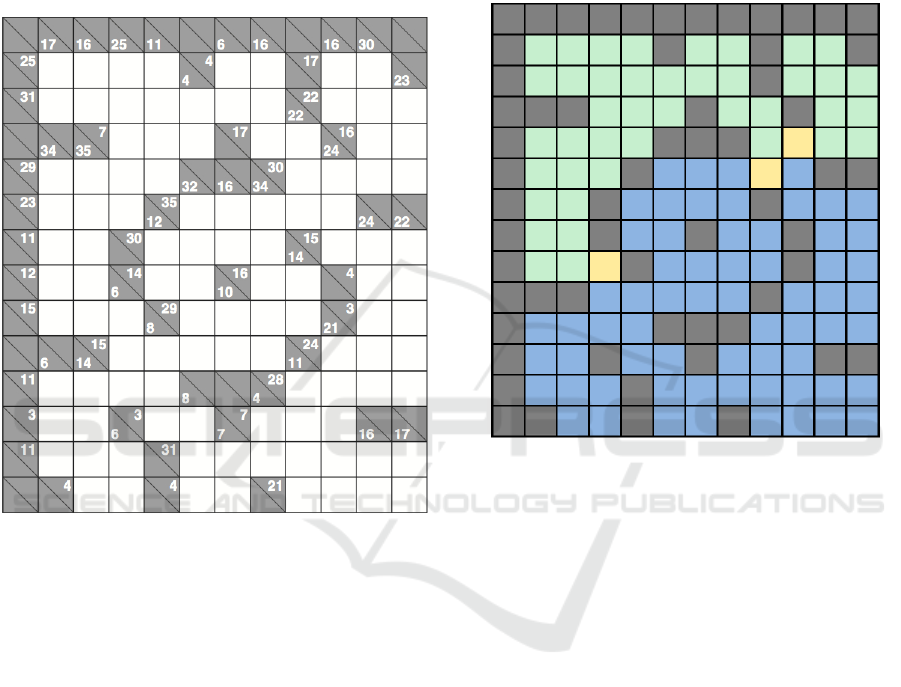
We consider the Kakuro shown in figure 1
which was published under the name ”Kakuro 1537
medium” in ”The Guardian” on February, 3rd, 2017.
Figure 1: Kakuro 1537.
The rules for Kakuro are ”Fill the grid so that each
run of squares adds up to the total in the box above or
to the left. Use only numbers 1-9, and never use a
number more than once per run (a number may reoc-
cur in the same row, in a separate run)”.
We modelled the problem with sum and
allDifferent constraints and could solve the problem
in less than a half second. To increase the size of
the problem we removed the numbers in the cells
(sums) and substituted them by variables. So we
have not anymore a Kakuro solver, we have a Kakuro
generator.
This offers us a problem with a high number of
solutions. We solved the problem with and without
use of the Meta CSOP approach.
We used a weight vector w = (1, 5) to prioritize the
minimization of the shared variables. In both cases
(using the Meta CSOP or not) we limited the total
time by 5 minutes. So the CSP without decomposi-
tion had 5 minutes to solve the problem, and the CSP
with decomposition approach had 5 minutes in total
(for the decomposition, solving of both sub-CSPs and
joining of the sub-CSPs). We used a decomposition
into two sub-CSPs. Important is that we do not do
anything in parallel. So we solved the two sub-CSPs
sequentially one after the other. This means that we
can use other parallelizations like search space split-
ting too, to increase the solving speed even more. Of
course we also can solve the sub-CSPs in parallel to
save a little bit less as the half total time.
Figure 2: Decomposition of the Kakuro.
Figure 2 shows the decomposition of the Kakuro
into two sub CSPs. The variables which are repre-
sented by the green cells are only in sub-CSP P
1
, the
blue cells only in sub-CSP P
2
. The yellow cells are
represented by shared variables which are in both sub-
CSPs. A decomposition into two sub-CSPs with only
three shared variables is an optimal solution for this
Kakuro.
The decomposition approach could find 14.91
times more solutions than the other, in the same time.
Remark: It is clear that not every CSP can be im-
proved with the Meta CSOP, but there are usecases,
like the Kakuro example shows. Future work should
investigate for which kind/ structure of CSPs this new
approach is especially useful.
5 CONCLUSION AND FUTURE
WORK
We have presented a new way to decompose a CSP
into sub-CSPs by the use of a Meta CSOP. The de-
composition is specialized to find distributed sub-
CSPs for parallel problem splitting with a minimum
ICAART 2019 - 11th International Conference on Agents and Artificial Intelligence
760

number of variables in each sub-CSP and a low num-
ber of shared variables between the sub-CSPs. We
evaluated our approach by a benchmark suite of Got-
tlob (Gottlob and Samer, 2009) . Our results have
shown that our approach is appropriate for partition-
ing a constraint network distribution on a given num-
ber of parallel constraint solving cores in short time.
In contrast to (Liu et al., 2018), the Meta CSOP works
also for big CSPs with more than 2000 variables and
constraints.
Future work will include a comparison with other
decomposition methods like (Karypis and Kumar,
1998) and their developments, and more practical
tests which will show the influence of the decomposi-
tion on the solving speed of the original CSP. Further-
more we will also focus on searching decomposition
methods which minimize the size of the shared do-
main sizes (i. e.
∏
∀x
i
∈{shared variable}
|D
i
|) and not only
the shared variables.
REFERENCES
Dechter, R. (2003). Constraint processing. Elsevier Morgan
Kaufmann.
Faltings, B. (2006). Distributed constraint programming.
In Handbook of Constraint Programming, pages 699–
729.
Gottlob, G., Leone, N., and Scarcello, F. (2000). A compar-
ison of structural csp decomposition methods. Artifi-
cial Intelligence, 124(2):243–282.
Gottlob, G. and Samer, M. (2009). A backtracking-based
algorithm for hypertree decomposition. ACM Journal
of Experimental Algorithmics, 13:1:1.1–1:1.19.
Hamadi, Y. (2002). Optimal distributed arc-consistency.
Constraints, 7(3-4):367–385.
Karypis, G. and Kumar, V. (1998). Multilevel algorithms
for multi-constraint graph partitioning. In Proceed-
ings of the ACM/IEEE Conference on Supercomput-
ing, SC 1998, November 7-13, 1998, Orlando, FL,
USA, page 28. IEEE Computer Society.
Liu, K., L
¨
offler, S., and Hofstedt, P. (2018). Hypertree de-
composition: The first step towards parallel constraint
solving. In Seipel, D., Hanus, M., and Abreu, S., edi-
tors, Declare 2017 – Conference on Declarative Pro-
gramming, pages 91 – 103.
Marriott, K. (1998). Programming with Constraints - An
Introduction. MIT Press, Cambridge.
Nguyen, T. and Deville, Y. (1998). A distributed arc-
consistency algorithm. Science of Computer Program-
ming, 30(1-2):227–250.
Prud’homme, C., Fages, J.-G., and Lorca, X. (2017). Choco
documentation.
R
´
egin, J., Rezgui, M., and Malapert, A. (2013). Embarrass-
ingly parallel search. In Principles and Practice of
Constraint Programming - 19th International Confer-
ence, CP 2013, Uppsala, Sweden, September 16-20,
2013. Proceedings, pages 596–610.
Rolf, C. C. and Kuchcinski, K. (2009). Parallel con-
sistency in constraint programming. In Proceed-
ings of the International Conference on Parallel and
Distributed Processing Techniques and Applications,
PDPTA 2009, Las Vegas, Nevada, USA, July 13-17,
2009, 2 Volumes, pages 638–644.
Rossi, F., Beek, P. v., and Walsh, T. (2006). Handbook of
Constraint Programming. Elsevier, Amsterdam, First
edition.
Tsang, E. P. K. (1993). Foundations of constraint satis-
faction. Computation in cognitive science. Academic
Press.
Yokoo, M. and Hirayama, K. (2000). Algorithms for
distributed constraint satisfaction: A review. Au-
tonomous Agents and Multi-Agent Systems, 3(2):185–
207.
Decomposing Constraint Satisfaction Problems by Means of Meta Constraint Satisfaction Optimization Problems
761