
Automated Vision System for Cutting Fixed-weight or Fixed-length
Frozen Fish Portions
Dibet Garcia Gonzalez
1
, Nelson Alves
1
, Ricardo Figueiredo
2
, Pedro Maia
3
and Miguel Angel Guevara Lopez
1,4
1
Computer Center Graphics, Minho University, Guimarães, Portugal
2
Gel Peixe, Loures, Portugal
3
Sociedade Industrial de Robótica e Controlo, S. A., Aveiro, Portugal
4
Centro Algoritmi, Minho University, Guimarães, Portugal
Keywords:
Computer Vision, 3D Reconstruction, Automation, Frozen Fish Automatic Cut, Optimization, Automated
Optical Inspection.
Abstract:
The increase in fish demand poses a challenge to the food industry that needs upgrades both for: (1) offering
new and diverse products and (2) optimizing it’s processing line throughput and at the same time guaranteeing
the fishes’ quality and appearance. This work presents an innovative computer vision system, to be integrated
into an automatic frozen fish cutting production line. The proposed system is able to perform the 3D recon-
struction in real time of every frozen fish, and allows to: (1) identify and automatically separate head bone,
body and tail parts of the fishes; and (2) estimate with high accuracy where cut the fishes’ body to produce
the wanted slices, according to requirements (parameters) of weight or width previously defined. The exper-
imental and statistical results are very promising and show the viability of the developed system. As main
contribution (novelty) this new method is able to estimate automatically and with high precision the weight of
the part corresponding to the body of the fishes and thus optimizing the cut of the fish slices. With this, we
expect to achieve a significant reduction of fish losses.
1 INTRODUCTION
Fishing is one of the sources of food, nutrition, fi-
nancial income and livelihoods for hundreds of mil-
lions of people around the world. The supply of fish
at worldwide level reached a record high of 20kg
per capita in 2014 (Food and of the United Nations,
2016). This increase in fish demand poses a chal-
lenge to the industry whose current approaches for
fish cutting are mainly based on manual work and cuts
are made using only fixed dimensions. On the other
hand, consumers want to buy fish by weight, without
scales and with a great visual appearance (freshness).
This demand, imposes a challenge to the food indus-
try that needs upgrades both for: (1) offering new
and diverse products and (2) optimizing it’s process-
ing line throughput and at the same time guaranteeing
the fishes’ quality and appearance.
Currently, food processing, as it is the case of fish,
tends to be carried out in industrial and automated en-
vironments (Booman et al., 2010). Currently, automa-
tion is more and more a reality due to the well known
advantages. The Automatic (Automated) Optical In-
spection (AOI) algorithms and methods are currently
part of the "automation" bundle and allows for preci-
sion, repeatability, and uninterrupted periods of work
during all the year.
This work presents a new computer vision system,
to be integrated into an automated processing line,
able to the three dimensional (3D) reconstruction of
frozen fish (in real time), and automatically segment
the fishes into three (defined) parts (i.e. head bone,
body and tail). Also, the developed system will esti-
mate with high accuracy where (attending to an estab-
lished reference coordinate system) to cut the fishes
slices according to requirements (parameters) such as
weight or width.
The AOI-based method proposed here is a tailor-
made solution developed for a specific client, a rep-
resentative player of the Portuguese and international
fish industry. This new system will allow to optimize
the cutting process, replacing the today current sce-
nario where a human operator is responsible for cut-
ting the frozen fish in a pre-determined and fixed di-
Gonzalez, D., Alves, N., Figueiredo, R., Maia, P. and Lopez, M.
Automated Vision System for Cutting Fixed-weight or Fixed-length Frozen Fish Portions.
DOI: 10.5220/0007482407070714
In Proceedings of the 8th International Conference on Pattern Recognition Applications and Methods (ICPRAM 2019), pages 707-714
ISBN: 978-989-758-351-3
Copyright
c
2019 by SCITEPRESS – Science and Technology Publications, Lda. All rights reserved
707
mension while at the same time inspects it for "de-
fects" (e.g. if it is the "head bone" present and visi-
ble?).
2 PREVIOUS WORK
The computer vision technologies applied to the in-
dustry cover a great variety of solutions for image
acquisition like: visible/near-infrared, computed to-
mography, X-ray (Kelkar et al., 2015), magnetic res-
onance imaging, laser scanner (Kelkar et al., 2011) in
2D and 3D space (Mathiassen et al., 2011). The es-
timation of weight using computer vision techniques
implies the determination of density. Magnetic res-
onance imaging, computed tomography, laser scan-
ners,and even X-ray are imaging modalities that have
been frequently employed for this kind of task.
An overview of some of the AOI-based developed
solutions for "food inspection", in specific, focused
to compute (estimate) parameters, such as the weight
and density are presented to follow.
In (Viazzi et al., 2015), computer vision tech-
niques are used to estimate the weight of a complete
fish. The study uses regression techniques to find the
best model that estimates weight using features ex-
tracted from images. The computer vision algorithm
includes four steps. First, detect the region that en-
closes the fish. Second, the fish is segmented using
the "Otsu adaptive thresholding" algorithm. Next, it
is removed the tail fin using a shape analysis method.
Finally, some features like height, length, and area are
extracted with and without including the tail fin. As
conclusions, authors state both for: 1) the area pa-
rameter is sufficient and more robust to estimate the
weight of a fish; and 2) the tail fin negatively influ-
ences the weight estimation. Another approach tries
to establish a relation between the projected area of
sushi shrimp, captured using an RGB camera, and its
corresponding weight (Poonnoy and Chum-in, 2012).
In (Mortensen et al., 2016) for the use case of
broiler chickens weight estimation, it is described a
system composed of a weighing platform (used to
give a reference weight) and a RGB-D sensor (Mi-
crosoft kinect), where authors developed an algorithm
including the following steps: (1) segment the broil-
ers using watershed and region growing techniques
in a previously filtered gray-scale image (combining
a Gaussian filter and morphological operators); (2)
the extraction of features like projected area, width,
perimeter, radius eccentricity, volume and others from
each segmented broiler; and (3) weight prediction of
each broiler based on the extracted features using ar-
tificial neural networks. A convex hull and numeri-
cal integration are used to obtain an approximated 3D
model of the broilers.
In (Adamczak et al., 2018) it is used a white light
(3D scanning) technology to determine the weight of
the chicken breasts.
Eggs volume estimation based on computer vi-
sion techniques was explored by (Soltani et al., 2015)
with the objective to extract the eggs major and minor
diameters. Two methods for estimating the volume
were tested: 1) a Mathematical model based on Pap-
pus theorem; and 2) Artificial Neural Networks. As
result, it was observed that the developed mathemati-
cal model achieved better results..
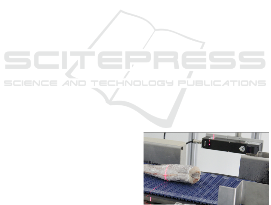
3 AUTOMATIC VISION SYSTEM
In order to support the development of the proposed
method, we built an experimental prototype (a stand
alone machine) comprising: 1) a conveyor belt that
moves at a speed of 0.5 m/s, which can transport
fishes of different sizes and volumes; 2) a precision
scale; 3) two "Entry-Level 3D Laser Line Profile Sen-
sors" - Gocators 2150 (Technologies, 2018) in an op-
posite layout placed at a distance of one meter (Fig-
ure 1). The Gocator 2150 is a 3D smart sensor / cam-
era, an all-in-one solution that lets factories to im-
prove efficiency in product validation; and 4) an in-
dustrial PC.
With this, each fish is weighted using the scale
and its total weight (T
w
) is recorded. Then, the fish
is scanned using the Gocators sensors, resulting two
line profiles (corresponding to both sides of the fish;
top and bottom). The computed profiles are then inte-
grated generating a precise 3D fish model using a fine
tuning developed computer vision algorithm.
Figure 1: Hardware prototype of the acquisition module,
including sensors that emits and capture lines of laser that
are projected in the fish body over the conveyor belt.
Taking as input the generated 3D model, we estimate
the individual weight of a voxel (V
w
) dividing the total
weigh of the fish (T
W
) by the total number of the com-
ICPRAM 2019 - 8th International Conference on Pattern Recognition Applications and Methods
708
puted voxels. A voxel is considered the minimum unit
of a 3D object (the fish in this case) with dimensions
w, l and h respectively. Additionally, it is computed
the total volume (T
V
) as the sum of all the volumes of
the voxels. The fish density (ρ) is calculated dividing
the total volume (T
V
) by the total weight(T
W
).
The cameras reference system is used as the global
coordinates system. Therefore, the two produced pro-
files are identified as the top and the bottom respec-
tively. The x axis coincides with the width (w), the z
axis with the height (h) and the y axis with the length
(l) of the fish.
The built 3D model is then segmented in three
parts: the head bone, body and tail fin models. The
head bone is considered waste and body and tail fin
are separated to be processed before introducing these
into the cutting system machine. In the next step, the
3D model of the body part is used as input to deter-
mine the optimal coordinates of slices for each in-
dividual fish, taking into account the previously se-
lected parameters (length or weight). The description
of the mechanical part of the cutting system machine
will not be discussed here, due to, it is not an objective
of this work.
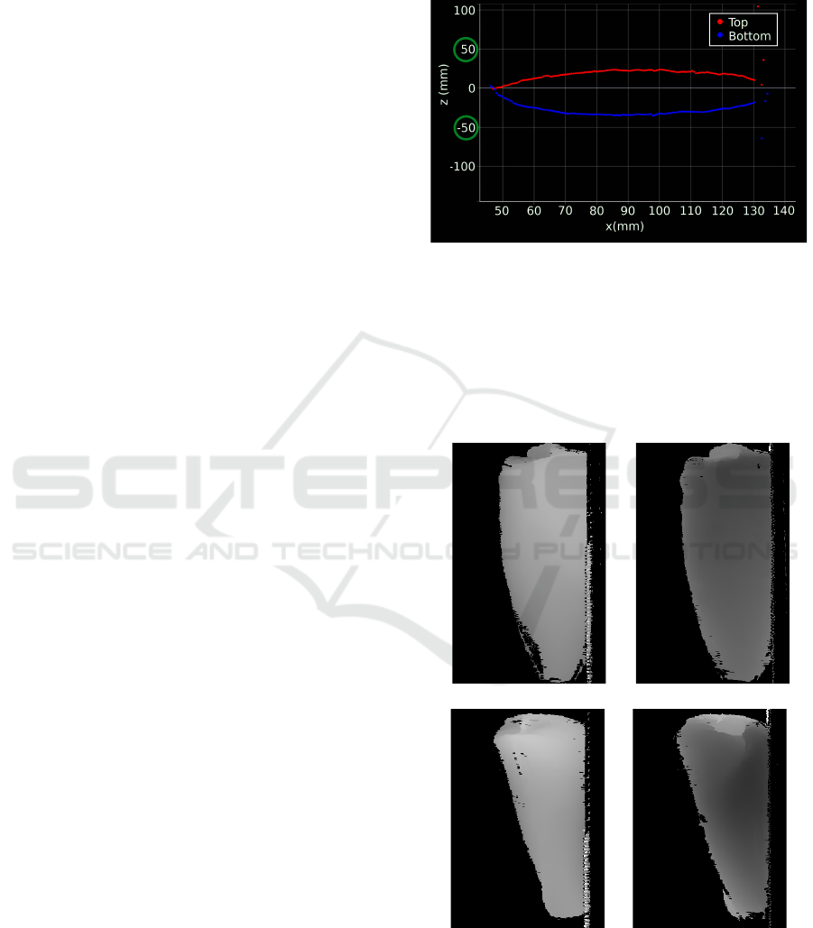
3.1 Data Acquisition and
Pre-processing
For the development of this work, we used an exam-
ple dataset comprising 200 fishes of Merluccius mer-
luccius with different sizes, supply by the "Gel Peixe"
company (http://gelpeixe.pt). The used sensors / cam-
eras (Gocator 2150) capture information such as: in-
tensity levels and depth profiles. However, we used
only, as input data, the top and bottom depth profiles
captured by the sensors, which are acquired when the
fishes are moving through the conveyor belt, inside
of the sensors field of view (the y axis). Cameras
are previously calibrated and aligned, guaranteeing
that the extrinsic parameters between both cameras
are known. An encoder is used to trigger the cameras
in a synchronized way. With this, we have a resolu-
tion that allows to capture voxels with the following
dimensions in mm: 1x1x0.6 (x,y,z) respectively.
The pre-processing step aims to remove every in-
formation that is not belong to the fish, such as the
foreign objects and the conveyor belt among others.
The foreign’ objects subtraction consists in the ap-
plication of a thresholding process to both profiles
(top and bottom) in which are correlated the width of
the conveyor belt and the maximum width of the fish.
The threshold was selected heuristically taking into
account the fish dimensions. It allows the selection
of a correct ROI (Region of Interest), which is criti-
cal for the execution of the next steps. The Figure 2
shows the measured profile from each camera and the
manual threshold selection.
Figure 2: Example of profiles: Top (red) and Bottom (blue).
Heuristically selected thresholds (enclosed in green circles).
While the fish is crossing the field of view of the cam-
eras, the profiles are captured and stored in order to
form two gray-scale images (Figure 3). These images
still need a filtering step in order to remove the con-
veyor belt and other noise related to the profile acqui-
sition.
(a) 2260gr (b) 2260gr
(c) 1880gr (d) 1880gr
Figure 3: Bottom (a, c) and top (b, d) images without the
filtering step
For this task, we employ mathematical morphology
operators combined with logical operations, as pre-
Automated Vision System for Cutting Fixed-weight or Fixed-length Frozen Fish Portions
709
sented to follow. These steps are applied to the bot-
tom ( f
b
) and top ( f
t
) two dimensional (2D) gray-scale
images.
1. Adjust the coordinate system.
f
t
(x,y) = f
t
(x,y) + min( f
b
(x,y)) (1)
f
b
(x,y) = f
b
(x,y) + min( f
b
(x,y)) (2)
where min( f
b
(x,y)) calculates the minimum (co-
ordinates in the z axis) value of the bottom profile.
2. Image binarization
b
t
(x,y) =
1 if f
t
(x,y) 6= 0
0 if f
t
(x,y) = 0
(3)
b
b
(x,y) =
1 if f
b
(x,y) 6= 0
0 if f
b
(x,y) = 0
(4)
3. Binary mask
m(x,y) = b
t
(x,y) ∨ b
b
(x,y) (5)
4. Improving the binary mask. It is applied a mor-
phological opening operation with structuring el-
ement K to m(x,y), with this are removed small
(noise) particles.
m(x,y) = (m(x,y) K(a,b)) ⊕ K(a, b) (6)
5. Gray image reconstruction
f
0
t
(x,y) = f
t
(x,y) × m(x, y) (7)
f
0
b
(x,y) = f
b
(x,y) × m(x, y) (8)
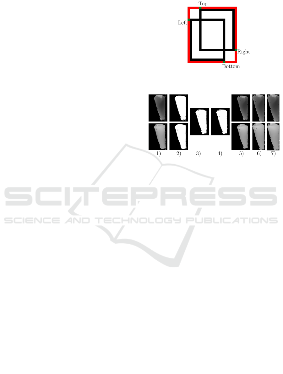
6. Blob (fish) detection and image cropping. In this
step we find the regions of interest (the fish) in
f
0
t
and f
0
b
. Then, the bounding boxes (rectangles)
that enclose each blob are superimposed in order
to form a new rectangle that is used in the crop-
ping process of f
0
t
and f
0
b
. An example can be
seen in Figure 4.
7. A Gaussian filtering is applied to reduce noise,
which allows to smooth the previously recon-
structed gray image.
The Figure 5 shows the image evolution since step
1 to step 7.
Figure 4: Rectangle estimation used in the cropping process
of f
0
t
and f
0
b
.
Figure 5: Image processing work flow (steps).
3.2 3D Model Reconstruction and
Density Estimation
The filtered top and bottom images are used as in-
put to build the 3D model. The corresponding row in
both images are used in the building of L new images
containing the edges (contours) of the region (area)
of the fish in each particular image (plane) (see Fig-
ure 6). Unconnected points are linked using a cubic
spline algorithm to close the fish area in each plane.
The number of pixels enclosed by this area is N
i=1..L
.
The total area (in mm
2
) is calculated using the equa-
tion:
A
i=1..L
= N
i
∗ w ∗ h (9)
The volume in mm
3
between two continuous im-
ages planes is computed as:
V
i=1..L
= A
i
∗ l (10)
The total fish volume (T
V
) in mm
3
is:
T
V
=
∑
i=1..L
V
i
(11)
Knowing the weight (T
w
) of each fish and its vol-
ume (T
V
) we can estimate its density ρ as:
ρ =
T
w
T
V
(12)
Finally, is calculated the weight associated to the
i
th
image as:
ICPRAM 2019 - 8th International Conference on Pattern Recognition Applications and Methods
710
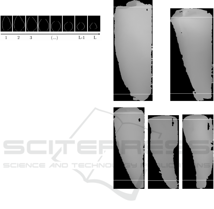
W
i=1..L
= V
i
∗ ρ (13)
Figure 6: Profile samples.
3.3 Fish Segmentation
The cutting process of frozen fish always involves a
first stage of bone cutting (i.e. the head bone). The
detection of the exact position where to cut the head
bone (L
bone
) is a trial and error process when done
manually. An experienced operator can make 2 to 3
cuts on the same fish before to achieve a first slice of
the fish with the expected (optimal) quality. To extract
the correct place (position) for cutting the head bone,
we developed a simple algorithm that takes as input
the images obtained in the step 7, as it can be observed
in the sub-section 3.1 (see Figure 5).
To automatically identifies the coordinates for cut-
ting the head bone, we developed an algorithm that
consists in moving a segment of line using an inclina-
tion angle of 30
◦
from the upper left edge downwards
in both images (top and bottom). This procedure is
repeated until (at least) the segment of line intersect
one of the pixels belonging to the fish, in any one of
the two images (top or bottom). The length of the tail
fin (L
tail
) depends on the size of the fish and the opti-
mization strategies (i.e. the length that was previously
defined by the costumer). With this, the body (L
u
) is
considered the part (portion) between head bone and
tail fin (space between L
bone
and L
tail
, which is the
"useful space" for cutting the slices of the fish. The
Figure 7 shows two segment of lines, which identified
(divide) the head bone, body and the tail fin section of
the fish.
3.4 Fish Cut Optimization Strategies
Once segmented the body of the fish, the next step is
related to computing the coordinates where its will
be produced the cuts for obtaining the optimized
fish slices. As required by the costumer, the fish
can be processed following one of two well-defined
strategies: 1) Fixed-Length, using as input a selected
length, between a range of values to cut the fish slices;
and 2) Fixed-Weight, using as input a selected weight
to cut the fish slices.
The Fixed-Length strategy allows a length range
between min
length
and max
length
to apply the cuts.The
(a) 2260gr (b) 1880gr
(c) 670gr (d) 520gr (e) 510gr
Figure 7: Bone estimation and tail fin section. The tail
length is fixed to 3cm.
goal is to minimize the waste, therefore, it can be in-
tended as the minimization of the distance between
the last slice coordinates and the start-off position of
the tail fin (L
tail
). For this purpose, we use the algo-
rithm 1. In our setup, we consider the size of the fish
as having L mm, due to the fish’s profiles coordinates
are acquired with a distance of 1 mm in the sense of
the y axis.
The algorithm 2 describes the Fixed-Weight strat-
egy.
Automated Vision System for Cutting Fixed-weight or Fixed-length Frozen Fish Portions
711
Algorithm 1: Fixed-Length strategy algorithm. The IF
condition allows adding 1mm more in another to consider
the loss produced by the saw.
Result: A vector with all the cuts positions
(positions)
L
u
= L − L
bone
− L
tail
;
cuts_number = 0;
rest_space = L
u
− cuts_number ∗ min_length;
while (rest_space > max_length) do
cuts_number + +;
rest_space =
L
u
− cuts_number ∗ min_length;
end
adding = rest_space/cuts_number;
real_cut_width = min_length + adding;
start = L
bone
;
positions = [];
for (i = 0;i < cuts_number;i + +) do
position_to_add = 0;
if (real_cut_width + 1 > max_length then
position_to_add = max_length;
else
position_to_add = real_cut_width + 1;
end
Insert position_to_add into the vector
positions;
start+ = position_to_add;
end
Algorithm 2: Fixed-Weight strategy algorithm.
Result: A vector with all the cuts positions
(positions)
start = L
bone
;
acc_weight = 0.0;
positions = [];
for (i = L
bone
;i < L
bone
+ L
u
;i + +) do
acc_weight+ = V
i
∗ ρ;
if (acc_weight >= desired_weight) then
position_to_add = i − start;
Insert position_to_add into the vector
positions;
start = i;
acc_weight = 0.0;
end
end
4 EXPERIMENTAL SETUP /
VALIDATION
In order to validate and verify the developed meth-
ods, we use the Merluccius merluccius dataset, a set
of fishes (with different weights), which were contin-
uously scanned, and volume of every fish in each it-
eration was computed. Then, statistical descriptors,
such as, the mean and standard deviation were ex-
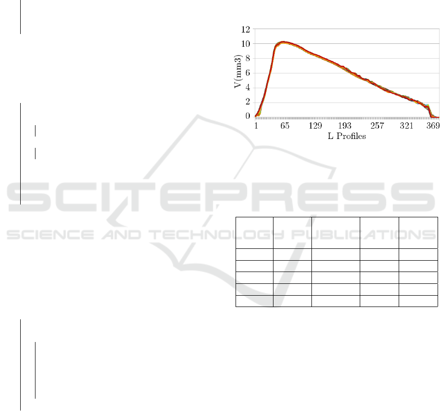
tracted. An example, using one fish can be observed
at Figure 8, which shows the volume profiles of a fish
(weighting 1880gr) computed 200 times in different
positions, using the Equation 10. The Table 1 shows
the statistical descriptors (mean and standard devia-
tion) computed 200 times in different positions using
five different fishes.
Figure 8: Volume behavior after scanning a 1880 gr fish 200
times.
Table 1: Computed statistical descriptors of the volume of
five fish of different weights. Each fish was measured 200
times.
Fish
Figure
7
Mean
(mm
3
)
Std. Dev.
(mm
3
)
Max
(mm
3
)
Min
(mm
3
)
a 2425,6 5,87 2436,6 2406,4
b 2059,7 10,67 2080,5 2031,8
c 740,76 7,02 751,5 724,37
d 590,46 2,23 601,6 589,42
e 555,34 3,47 561,1 546,65
In the Table 1, It can be observed that computed
volumes have low variability. Only in the case of fish
2 the standard deviation (Std.Dev.) was superior to
10mm
3
. Another observed result is the fact that high
volume variability is not related to the fish volume.
The use of the density calculated in the Equa-
tion 12 and its use in the estimation of the voxel
weight (V
w
) is validated. For this, we take into ac-
count the customer restrictions. Specifically, the fact
that the weight deviation should not exceed the ±10gr
range, when it is selected the fixed weight strategy
(i.e. cut all slices using a fixed / previously selected
weight).
To test if this specification is respected, we apply
the following steps:
• Scan one selected fish to determine each V
i
.
ICPRAM 2019 - 8th International Conference on Pattern Recognition Applications and Methods
712
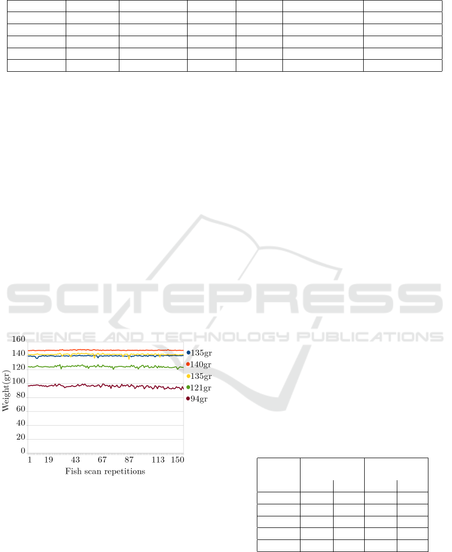
Table 2: The behavior of the weight for an 803 gr fish cut in 5 peace. 150 measures by each fish.
Weight (gr) Mean (gr) Std. Dev. (gr) Max (gr) Min (gr) Max-Weight (gr) Weight-Min (gr)
135 138,25 0,71 139,29 136,51 4,29 -1,51
140 145,35 0,38 146.41 144,53 6,41 -4,53
135 139,31 1,12 141.18 135,47 6,18 -0,47
121 124,84 1,20 127.75 120,83 6,75 0,17
94 96,44 1,80 99.90 91,36 5,90 2,64
• Weight the fish (T
w
) and calculate the density us-
ing the Equation 12.
• Using the ρ and V
i
, calculate the W
i
(Equation 13)
that is the weight associated to the i
th
image (see
Figure 6).
• Cut the fish at random places and measure the
slice length and weight using a rule and a preci-
sion scale.
• Using the length of the fish slice, estimate the
weight accumulated by each slice weight of the
profiles (W
i
).
Results can be seen in Figure 9. It shows 5 slices ob-
tained from a fish with 803gr of weight. We have
calculated the individual weight of each slice and
scanned 150 times. The Table 2 shows the minimum
and maximum obtained weight measured for each in-
dividual slice. In the two last columns, it is observed
that the weight of each individual slice has values that
are less than the established limit (±10gr).
Figure 9: Estimated weight of one fish of 803gr cut in
135gr, 140gr, 135gr, 121gr and 94gr.
From the Table 2, it can be deduced that the esti-
mated weights most of the times are greater than the
real weight of the fish slice. This does not represent
a problem for the proposed algorithms, because they
take into account the waste produced by the cutting
saw. With this, after cutting the fish, the actual weight
of the obtained slices is slightly lower than the esti-
mated weight. The volume lost at the time of cutting
is always less than W
j
and will depend on the thick-
ness of the cutting saw used and the fish’s area at the
cutting position.
The waste produced by the cutting saw near to the
tail fin is smallest than the wasted produced near to
the head bone. As a positive aspect, in all cases, even
without considering the waste produced by the cutting
saw, always the final weights are in the desired range
of ±10gr - the customer accepted deviation in relation
to the desired weight.
Taking in consideration the needs of the client,
the final system prototype has been adjusted to pro-
duce more than 70 slices by minute. For this purpose,
the developed system has been optimized to exploit
the power of multicore CPUs by leveraging the use
of a multi-thread architecture. One thread control the
cameras to acquires the fish profiles and building the
top and bottom images, and the rest (the free threads)
are used for algorithms processing. This approach
provides real-time processing, and is able to guaran-
tee the customer’s requirements concerning the num-
ber of fishes slices / minute.
The total delay of the automated vision system
is the sum of the acquisition time and the process-
ing time (see Table 3). Each fish takes between half
second and a second to be processed. In huge fish,
sometimes, the individual processing time of a fish is
slightly bigger than one second. With this, it can be
concluded that the automated vision system can per-
form almost in real time system.
Table 3: Behavior of acquisition and processing times for
different sizes of fish in milliseconds (ms).
Weight
(gr)
Acquisition
Time (ms)
Processing
Time (ms)
Max. Min. Max. Min.
2260 821 717 294 170
1880 749 671 286 129
670 681 610 217 54
520 451 440 98 49
510 422 410 82 46
Automated Vision System for Cutting Fixed-weight or Fixed-length Frozen Fish Portions
713

5 CONCLUSIONS
The main contribution of this work is the develop-
ment of an automated real time computer vision sys-
tem able to: 1) capturing and building a precise 3D
representation of frozen fishes; and 2) accelerating the
automated frozen fish cutting in the production lines
at industrial level. An innovative high performance
image processing method has been developed that al-
lows to automatically infer the optimal place (coordi-
nates) where to cut the fish portions, attaining a pre-
viously wanted / selected weight or length of the pro-
duced slices and thus reducing the waste during the
cutting process. While the dataset used is still small,
the experimental statistical results demonstrated that
the proposed system prototype is feasible to be imple-
mented and validated in real industry environments.
6 FUTURE WORKS
The future work aims to validate the developed com-
puter vision system in real production lines. Also, it
is planned to improve the developed system with the
ability to evaluate the freshness of the produced fish
portions by analyzing properties like color, shape and
texture.
ACKNOWLEDGMENT
This article is one of the results associated to the
project MaxCut4Fish: Research and Development of
an Intelligent System for Automatic and Optimized
Cutting of Frozen Fish (project n
o
017664), sup-
ported by the European Regional Development Fund
(ERDF), through the Competitiveness and Interna-
tionalization Operational Program (COMPETE 2020)
under the PORTUGAL 2020 Partnership Agreement.
REFERENCES
Adamczak, L., Chmiel, M., Florowski, T., Pietrzak, D.,
Witkowski, M., and Barczak, T. (2018). The use of
3d scanning to determine the weight of the chicken
breast. Computers and Electronics in Agriculture,
155:394 – 399.
Booman, A., Márquez, A., Parin, M. A., and Zugarramurdi,
A. (2010). Design and testing of a fish bone separator
machine. Journal of Food Engineering, 100(3):474 –
479.
Food and of the United Nations, A. O. (2016). The state of
world fisheries and aquaculture (sofia).
Kelkar, S., Boushey, C. J., and Okos, M. (2015). A method
to determine the density of foods using x-ray imaging.
Journal of Food Engineering, 159:36–41.
Kelkar, S., Stella, S., Boushey, C., and Okos, M. (2011).
Developing novel 3d measurement techniques and
prediction method for food density determination.
Procedia Food Science, 1:483 – 491. 11th Interna-
tional Congress on Engineering and Food (ICEF11).
Mathiassen, J. R., Misimi, E., Bondø, M., Veliyulin, E., and
Østvik, S. O. (2011). Trends in application of imag-
ing technologies to inspection of fish and fish prod-
ucts. Trends in Food Science & Technology, 22(6):257
– 275.
Mortensen, A. K., Lisouski, P., and Ahrendt, P. (2016).
Weight prediction of broiler chickens using 3d com-
puter vision. Computers and Electronics in Agricul-
ture, 123:319–326.
Poonnoy, P. and Chum-in, T. (2012). Estimation of sushi
shrimp weight using image analysis technique and
non-linear regression models. Internation Conference
of Agricultural Engineering (CICGR-AGENC).
Soltani, M., Omid, M., and Alimardani, R. (2015). Egg vol-
ume prediction using machine vision technique based
on pappus theorem and artificial neural network. Jour-
nal of Food Science and Technology, 52(5):3065–
3071.
Technologies, L. (2018). Gocator 2100 series.
https://lmi3d.com/products/gocator/g2/2100-series.
Last accessed 13 November 2018.
Viazzi, S., Hoestenberghe, S. V., Goddeeris, B., and Berck-
mans, D. (2015). Automatic mass estimation of jade
perch scortum barcoo by computer vision. Aquacul-
tural Engineering, 64:42 – 48.
ICPRAM 2019 - 8th International Conference on Pattern Recognition Applications and Methods
714
