
Pattern Matching in Discrete Models for Ecosystem Ecology
Cinzia Di Giusto
1
, C
´
edric Gaucherel
2
, Hanna Klaudel
3
and Franck Pommereau
3
1
Universit
´
e C
ˆ
ote d’Azur, CNRS, I3S, France
2
AMAP - INRA, CIRAD, CNRS, IRD, Universit
´
e Montpellier, France
3
IBISC, Univ Evry, Universit
´
e Paris-Saclay, Evry, France
Keywords:
Rewriting Systems, Similarity Rate, Pattern Matching, Ecosystems.
Abstract:
In this paper we consider discrete qualitative models of ecosystems viewed as collections of interacting living
(animals, plants. . . ) and nonliving entities (air, water, soil. . . ), whose conditions of appearance/disappearance
are controlled by a set of formal rules (i.e., processes). We present here a rule-based method allowing to
compare ecosystems. The method relies on a measure of similarity and on an optimization algorithm. In
addition, the proposed method allows to detect patterns (i.e., ecological processes or sets of processes) in
ecosystems. We have validated the method by applying it against a set of models and patterns provided by
ecologists.
1 INTRODUCTION
Ecosystems are defined by complex processes of
highly different nature: e.g. bio-ecological, physico-
chemical and socio-economical. The dynamics of
such systems is difficult to grasp as it is the result of
an intricate interplay between a large number of pro-
cesses: the functioning of living species (fauna and
flora) and the dynamics of soil and climate. In ad-
dition, all these entities and processes are influenced
and often highly impacted by human activities.
Understanding the functioning of ecosystems is
thus crucial for a more sustainable management of
them. Indeed, we face today fast and dangerous
changes of most ecosystems (due to climate change,
to human activities. . . ) that we are compelled to un-
derstand so to appropriately react. Unfortunately, in
practice, the development and analysis of models of
ecosystems remain a challenge and constitutes a crit-
ical bottleneck as they are usually treated on a case-
by-case basis with few generalizations.
One relevant way of improving our understand-
ing of ecosystems functioning is to provide more for-
mal frameworks. They have proven to be valuable
for speeding up and better controlling the decision
procedures. Similarly to what happens in biology,
ordinary differential equations (ODE) are the dom-
inant modeling methodology for ecosystems (May,
1972, Lotka, 1925). The drawbacks of such models
are that: i) they usually need to quantify various pa-
rameters (mostly unknown). ii) They are not able to
faithfully represent the time scale required for obser-
vation of ecological processes which is usually large.
iii) On top of this, analytic solutions usually do not
exist and models often represent averaged and some-
times unrealistic behaviors of ecosystems. In contrast,
while discrete qualitative models are high level ab-
stractions of observed processes, they allow unrav-
eling the tangled causal relationships between sys-
tem’s entities (i.e. material constitutive components).
The success of discrete qualitative approaches is wit-
nessed, for instance, in systems biology with for-
malisms like Petri nets (Baldan et al., 2010), Boolean
networks (Thomas, 1973), process algebras (Cardelli,
2005) and rewriting systems (Giavitto et al., 2004), to
cite a few.
In ecology, discrete qualitative modelling is still
pioneering and under exploited. Approaches such
as (Gaucherel et al., 2012, Gaucherel et al., 2014),
where the authors study the driving rules needed to
change agricultural mosaics and model contrasted
landscapes, are promising. However, much more may
be obtained by developing original solutions based on
the suitable application of existing theory and associ-
ated (automated) tools. One of the goals of this paper
is to contribute in this regard.
As a starting point of our developments we take
a general discrete qualitative formalism proposed in
(Gaucherel and Pommereau, 2017). Ecosystems are
modeled as a set of (living and nonliving) entities
Di Giusto, C., Gaucherel, C., Klaudel, H. and Pommereau, F.
Pattern Matching in Discrete Models for Ecosystem Ecology.
DOI: 10.5220/0007485801010111
In Proceedings of the 12th International Joint Conference on Biomedical Engineering Systems and Technologies (BIOSTEC 2019), pages 101-111
ISBN: 978-989-758-353-7
Copyright
c
2019 by SCITEPRESS – Science and Technology Publications, Lda. All rights reserved
101

together with a set of rewriting rules expressing the
conditions of their appearance/disappearance (i.e., the
ecosystem component responses). These rules may
be interpreted as the functioning bricks of landscape
modelling. Each rule is, thus, part of a broader pro-
cess describing the behavior of the whole ecosystem.
Yet, there are processes that are common to sev-
eral ecosystems: e.g.–for species interactions– preda-
tion, competition, symbiosis. . . and it is crucial to be
able to identify them to better describe the ecosys-
tem under study. Hence, we can raise the following
questions: How can we detect whether a given pro-
cess is present in an ecosystem? Is the introduction
of a new entity causing the appearance of a known
process? Indeed, to detect wanted or unwanted inter-
action patterns would guide decisions for taking ac-
tions according to the management objectives, such
as preventing or reinforcing some ecosystemic pro-
cesses or states. Identify certain ecological processes
or interaction patterns –in a more computer science
oriented terminology– by employing classical graph-
theoretical methods on the state space is ineffective.
Indeed, in realistic ecosystem models, the modeled
dynamics usually leads to huge state spaces (often
hundreds of thousands of states). It is more efficient
to search for patterns by referring only to the (limited)
syntactical system specification as similar processes
look similar at the rule level.
From a more general point of view, a pattern
search corresponds to a variant of the problem of as-
sessing the similarity between models of ecosystems.
In order to compare two models of ecosystems, we
introduce a pair of mappings, the first identifying en-
tities and the latter rules, and a similarity measure ex-
pressed as a scoring function. This scoring majors
the number of matched entities and rules, and penal-
izes those that do not perfectly match. Similarity is
then defined as an optimization problem through the
scoring function. Indeed, the scoring function with
optimal value uniquely determines the mappings of
entities and rules. This way the definition of the scor-
ing function is used to search for interaction patterns
in the rule-based models of ecosystems. As the com-
plexity of this kind of search is exponential, it is not
always possible in realistic cases to find optimal solu-
tions in a reasonable time. Nevertheless, optimization
tools generally allow obtaining a sub-optimal solution
quite efficiently, solutions that can then be refined.
We implemented a prototype that allows encod-
ing the matching of two models into a pseudo-
Boolean optimization problem and invoking tool
Sat4j (Le Berre and Parrain, 2010) to solve it. We
applied this prototype to systematically match a col-
lection of predefined interaction patterns against a set
of models of “real” ecosystems.
The paper is structured as follows: Section 3 in-
troduces the formal modeling of ecosystems we have
used and presents running examples. Section 4 de-
fines similarity measures used to compare ecosystems
and discusses possible extensions of them. Several
comparisons between ecosystems are used as illustra-
tions for the scoring function. In Section 5, we present
the results of our main case study: a search of inter-
action patterns in realistic ecosystems. Next section 2
is devoted to an overview of related work, while some
concluding remarks and perspectives are presented in
Section 6.
2 RELATED WORK
The model of ecosystems developed in this paper
is an instance of the more general family of rewrit-
ing systems (Terese, 2003). Such systems have been
shown convenient in formalizing models, in particu-
lar for systems biology and chemistry. In these do-
mains, we thus find formalizations that are reminis-
cent of ours: the Biocham (Fages and Soliman, 2008),
the κ-calculus (Danos and Laneve, 2004), reaction
systems (Ehrenfeucht and Rozenberg, 2007), activity
networks (Delaplace et al., 2018), P-systems (Paun
et al., 2011), cellular automata (Gaucherel, 2006, Ag-
nihotri and Sharma, 2015) that describe the evolution
of cells and/or molecules applying rewriting rules.
Yet, the question of similarity appears rather novel
in rewriting systems. In a broader context, it is usu-
ally associated to the notion of equivalence. In con-
current systems like ours, equivalences are usually se-
mantics based, notable examples are partial ordering
equivalences, trace equivalence (van Glabbeek and
Goltz, 1989), bisimulation (Sangiorgi, 2011), prin-
cipal transition sequences (Wang et al., 2010), etc.
These notions are usually explored in theory and tai-
lored to highly abstracted languages, moreover com-
puted with a few existing tools. In practice, we can-
not expect to use such approaches on the huge state
spaces generated from detailed and realistic (qualita-
tive) models of ecosystems.
Works that are closer to ours can therefore be
found in domains in which models use structural as-
pects rather than their behaviors. For instance in
systems biology, several similarity measures can be
found (a good survey summarizing the used tech-
niques may be found in (Henkel et al., 2018)). Tech-
nically speaking, these methods include the anal-
ysis of similar pathways through a structural ap-
proach, namely the search of t-invariants in Petri net
models (Baldan et al., 2013a, Baldan et al., 2013b,
BIOINFORMATICS 2019 - 10th International Conference on Bioinformatics Models, Methods and Algorithms
102

Grafahrend-Belau et al., 2008). They also define a
similarity score, but our goal and underlying mod-
elling are considerably different.
Another domain that focuses on similarity rates
is business process modeling. For instance in (Xiao
et al., 2009), the authors evaluate the similarity of
Petri nets by comparing the set of structural elements
such as places and transition arcs. Similarity is based
on rates of identical elements. Instead, our approach
is finer-grained and more flexible: the mappings al-
low different names of entities and rules, and we allow
partially matched rules. In (Bae et al., 2006), process-
based models are studied and similarity is defined on
sets of nodes as the proportion of matched ones. Yet,
these authors do not deal with relations between them.
Likewise, in (Dijkman et al., 2011), other similarities
are explored. In this context the authors still compare
structural elements of workflows (e.g. sets of nodes),
but they allow different kinds of distance measures:
string-edit distance, labels synonyms and contextual
similarity. The latter measure is the closest to ours,
as we consider separately the input (or conditions, the
left hand side of a rule) and the output (realization, the
right hand side of a rule) of a node. Conversely, here,
we take into consideration penalties for elements that
are not matched. The work in (Dijkman et al., 2011)
shows how similarities in business process model are
linked to the semantic web domain, a survey of which
on corresponding metrics can be found in (Euzenat
and Shvaiko, 2007).
Finally, concerning explicitly the pattern search,
the work in (Milo et al., 2002) has analogous goals.
These authors search for patterns by counting the
number of occurrences of a given subgraph in spe-
cific networks (world wide web, electronic circuits,
. . . ) and comparing it to the number of occurrences in
random generated networks. This approach is com-
pletely different to ours, as their method applies to
graphs while ours applies to “hyper-graphs”. More-
over, they use techniques from statistics while we do
not.
3 MODELED ECOSYSTEMS
In this section, we recall the formal definition of a
model of an ecosystem as given in (Gaucherel and
Pommereau, 2017). An ecosystem consists of a set of
entities E that can be present (On) or absent (Off). We
assume that no entity may be simultaneously On and
Off. The status (the presence) of an entity a is called
polarity, we use a+ to denote that a is On, a− to de-
note that a is Off. The set of entities E with polarities
p ∈ {+, −} is E
p
= {a+,a− | a ∈ E}. The presence of
those entities is regulated by a sets of rewriting rules
R. More formally:
Definition 1 (Ecosystem). An ecosystem E is a tuple
(E,R) such that:
• E is a set of entities,
• R is a set of rewriting rules of the form r :
α
+
,α
−
ω
+
,ω
−
, where r is the name of the rule,
α
+
and ω
+
are sets of entities that are On, and α
−
and ω
−
are sets of entities that are Off.
We denote by lhs(r) (respectively rhs(r)) the set
of entities in the left (respectively right) hand side of
the rule r.
An ecosystem state s is defined by the information
about the presence or absence of all its entities. It is
described as the set of entities that are currently On:
thus s ⊆ E, and we assume that the remaining entities
E \ s are Off.
The dynamics of an ecosystem (E,R) is paramet-
ric over its initial state s
0
. It comprises all reachable
states obtained by asynchronously applying the rules
in R, in a non-deterministic way. A rule r is enabled
at a state s if the rule’s left hand side, i.e., (α
+
,α
−
),
matches the entities defining s. It means that α
+
⊆ s
and α
−
∩s =
/
0. If it is the case, the rule may apply and
a new state s
0
is generated by updating s according to
the rule’s right hand side: s
0
= (s \ ω
−
) ∪ ω
+
.
Example 1 (Pond). We consider a toy-model of a
pond populated with two species of fish, piscivorous
and insectivorous ones. The pond behavior is de-
scribed by the following rules:
1. if the pond disappears, all fish species disappear
too,
2. in summer the pond dries and disappears,
3. if the pond is not dried, both species of fish may
live in it,
4. if the piscivorous fish are present, insectivorous
fish disappear,
5. if insectivorous fish disappear, piscivorous fish
disappear too.
It consists of four entities: the summer, the pond,
and two kinds of fish (piscivorous and insectivorous);
and seven rules (see Table 1): Rules 1–5 correspond
to items 1–5 above, and rules 6 and 7 are used to
simulate the change of the seasons.
As an example of the dynamics, let s
0
= {P} be
the initial state. Then rule 3 is enabled and its appli-
cation gives s
0
= {P,IF,PF}. The whole dynamics is
then a directed graph whose vertices are the reach-
able states and whose edges correspond to the appli-
cation of rules.
Pattern Matching in Discrete Models for Ecosystem Ecology
103

Table 1: Entities and Rules for Example 1.
entities:
Su: Summer
P: Pond
PF: Piscivorous Fish
IF: Insectivorous Fish
rules:
1: P− PF−, IF−
2: Su+ P−
3: P+ PF+, IF+
4: PF+ IF−
5: IF− PF−
6: Su+ Su−
7: Su− Su+
Example 2 (Pesticides). As a second small example,
consider a fragment of another ecosystem with four
entities: birds, insects, pesticides and rain.
Table 2: Entities and Rules for Example 2.
entities:
B: Birds
I: Insects
Pe: Pesticide
R: Rain
rules :
1’: B+ I−
2’: I− B−
3’: Pe−, R+ I+
4’: Pe+ I−
5’: R+ Pe−
6’: B−, Pe− I+
The ecosystem is governed by the following prin-
ciples: birds eat insects and if insects disappear, birds
will vanish as well. As a disturbing factor we add
pesticides that may kill insects. Pesticides are washed
away by the rain and when there are no pesticides
and it is still raining, insects proliferate. Similarly
insect proliferation happens when there are no pes-
ticides and no birds. We do not take into account
in this example, all the rules (and possibly entities)
that are necessary to regulate the presence/absence
of rain. Entities and rules are given in Table 2.
4 SIMILARITY BETWEEN
ECOSYSTEMS
As mentioned in the introduction, our objective is to
identify interaction patterns. An interaction pattern
can be considered as a “tiny” ecosystem restricted to
few entities and rules. Thus it may be formalized in
the same syntax as the one for the whole ecosystem.
For example, the “habitat” interaction pattern is com-
posed of one entity featuring a specific environment
(aquatic, terrestrial, pond, . . . ) and several entities in-
habiting this environment:
1. if the environment disappears, all inhabitants dis-
appear as well.
Similarly, an interaction pattern for the “predation”
process is composed of two entities and two rules
only:
1. if predators are present, then prey disappear,
2. if prey disappear, then predators disappear too.
In the example of the pond ecosystem, instances
of both above patterns are present. The predation in-
stance is composed of piscivorous and insectivorous
species, and of rules 4 and 5; while the habitat in-
stance is composed of entities pond, piscivorous and
insectivorous species and of rule 1. Table 3 shows a
formal representation of the predation pattern.
Table 3: Interaction pattern for predation pattern.
entities:
Pred: Predator
Prey: Prey
rules:
1
00
: Pred+ Prey−
2
00
: Prey− Pred−
We may observe that there is a syntactical “simi-
larity” between rules 4 and 5 in the pond ecosystems
and rules 1 and 2 in the predation pattern.
The concept of similarity will be the basis of
our investigation. Similarity is discussed in theory
(see for instance the philosophical work in (Tversky,
1977)) and also used in practice: in law (Mooiman,
2015), in natural sciences (Henkel et al., 2018) and
in various branches of computer science. Intuitively,
we express it in terms of how many groups of compo-
nents with the same roles are present in both ecosys-
tems. This means that, given two mappings, be-
tween entities and rules respectively, the similarity
rate is defined as the number of mapped entities plus
how many mapped entities the rules have in common.
More formally, let E
1
= (E
1
,R
1
) and E
2
= (E
2
,R
2
)
be two ecosystems, and µ and ρ be two mappings be-
tween entities and rules respectively. The first one is
µ : E
p
1
→ E
p
2
. The mapping µ is injective but not nec-
essarily total and polarities are consistent: i.e., if a+
is matched with b− then b+ is matched with a−. It is
encoded as a rectangular matrix X of size (|E
p
1
|×|E
p
2
|)
of Boolean values defined for each pair of entities
with polarities (m,n) ∈ E
p
1
× E
p
2
as
X
m,n
= 1 if µ(m) = n, 0 otherwise.
BIOINFORMATICS 2019 - 10th International Conference on Bioinformatics Models, Methods and Algorithms
104

a+
a−
...
b+
b−
.
.
.
∑
≤1
∑
≤1
∑
≤1
∑
≤1
(a) The encoding into matrix X of the mapping µ
for entities and the illustration of corresponding
restrictions.
u
1
...
v
1
.
.
.
∑
≤1
∑
≤1
(b) The encoding of matrix Y of the mapping ρ for
the rules and the corresponding restrictions.
Figure 1: Encoding of mappings µ and ρ.
In order to implement injectivity and the corre-
spondence between polarities we introduce three re-
strictions (see Figure 1a):
1. There is at most one “1” in each line:
∀m ∈ E
p
1
:
∑
n∈E
p
2
X
m,n
≤ 1;
2. There is at most one “1” in each column:
∀n ∈ E
p
2
:
∑
m∈E
p
1
X
m,n
≤ 1;
3. Polarities are consistently matched:
∀a ∈ E
1
,b ∈ E
2
:
X
a+,b−
= X
a−,b+
∧ X
a+,b+
= X
a−,b−
.
Likewise, the mapping ρ : R
1
→ R
2
maps the rules.
Similarly as for entities, it is encoded as a rectangu-
lar matrix Y of size (|R
1
| × |R
2
|) of Boolean values
defined for each pair of rules (u,v) ∈ R
1
× R
2
as
Y
u,v
= 1 if ρ(u) = v, 0 otherwise.
It is subjected to the following restrictions that
implements injectivity (see Figure 1b):
1. There is at most one “1” in each line:
∀u ∈ R
1
:
∑
v∈R
2
Y
u,v
≤ 1;
2. There is at most one “1” in each column:
∀v ∈ R
2
:
∑
u∈R
1
Y
u,v
≤ 1.
For each pair of mappings (µ,ρ) between ecosys-
tems E
1
and E
2
we define a scoring function S. The
function assesses the quality of the matching rules
with respect to the number of matching entities. The
simplest way to express the score is to count, for each
pair of matching rules ρ(u) = v (i.e., Y
u,v
= 1), the
number of matching entities through function µ on
both the left and right hand side (i.e., for each pair
of entities n and m in rules u and v respectively, we
count the sum of all X
n,m
= 1). The scoring function
is a ratio between previous sum and a constant that
counts the number of rules times the maximal num-
ber of entities in a rule. More precisely:
S
0
(X,Y ) =
1
T · r
·
∑
u ∈ R
1
,
v ∈ R
2
Y
u,v
·
∑
n∈u,m∈v
X
n,m
where r = min(|R
1
|,|R
2
|) is the cardinality of the set
of rules in the ecosystem having the smallest num-
ber of them, and T = max
u∈R
1
∪R
2
(|lhs(u)| + |rhs(u)|)
is the maximal number of entities in a rule in both
ecosystems, considering at the same time the left
(lhs(·)) and right (rhs(·)) hand side. However this
simple scoring does not take into account:
1. the different contribution of the left and right hand
side. This means, for instance, that a good match-
ing on the left hand side can compensate a bad
matching on the right hand one;
2. the proportion of entities that are not matched.
Scoring function S
0
does not differentiate between
two rule mappings that for a rule in one ecosystem
match the same number of entities but the size of
matched rules in the second system is different.
Example 3. For example, take the ecosystems R
1
with
one rule r
1
: A+, B+ C+ and R
2
with two rules
r
2
: A+, B+ C+ and r
3
: A+, B+,D− C+ . The
score for ρ
1
mapping r
1
to r
2
should be greater than
ρ
2
mapping r
1
to r
3
as in the latter the mapping is less
perfect and there are entities that are not matched.
We thus propose a better formulation for the scor-
ing function that takes into account these remarks.
The scoring function is now the sum of the scores of
Pattern Matching in Discrete Models for Ecosystem Ecology
105

the left hand side and the right hand side and can be
summarized as follows:
S(X,Y )
df
=
1
r · (L + R)
·
∑
u∈R
1
,v∈R
2
Y
u,v
(left(u, v) + right(u,v))
where r = min(|R
1
|,|R
2
|) as above, L =
max
u∈R
1
∪R
2
(|lhs(u)|) and R = max
u∈R
1
∪R
2
(|rhs(u)|)
are the maximal numbers of entities occurring in the
left (respectively right) hand side of the rules from
both ecosystems, and left(u,v) and right(u,v) are the
scores for each pair of matching rules u ∈ R
1
and
v ∈ R
2
:
left(u, v) =
∑
n∈lhs(u),
m∈lhs(v)
X
n,m
−
min(|lhs(u)|,|lhs(v)|) −
∑
n∈lhs(u),
m∈lhs(v)
X
n,m
− abs(|lhs(u)| − |lhs(v)|)
= 2 ·
∑
n∈lhs(u),
m∈lhs(v)
X
n,m
− min(|lhs(u)|,|lhs(v)|)
− abs(|lhs(u)| − |lhs(v)|)
right(u, v) = 2 ·
∑
n∈rhs(u),
m∈rhs(v)
X
n,m
− min(|rhs(u)|,|rhs(v)|)
− abs(|rhs(u)| − |rhs(v)|)
The construction of this scoring function is de-
picted in Figure 2 below. The part left(u, v) takes the
number of matching entities
M
L
=
∑
n∈lhs(u),m∈lhs(v)
X
n,m
and subtracts two penalties. The first one:
min(|lhs(u)|,|lhs(v)|) − M
L
corresponds to the max-
imum number of entities, which could be matched
minus those that are actually matched. The second
one: abs(|lhs(u)| − |lhs(v)|) expresses the number of
entities which could never be matched because of the
difference in the length of the left hand sides of the
two rules. This score is maximal when left(u,v) =
min(|lhs(u)|,|lhs(v)|) and |lhs(u)| = |lhs(v)|, i.e., the
left hand sides of u and v have the same length, and all
their entities match. The part for the right hand sides
is defined analogously. The overall score is normal-
ized with respect to the number of rules r times L plus
R. As an effect of penalties, the score can be negative
but it is always between -1 and 1.
Similarity is then defined with respect to the scor-
ing function, as the maximal value it can have with
respect to all the possible mappings µ and ρ. It is pos-
sible to enumerate all solutions having a score greater
than a given threshold.
Also, depending on the specific objective, coeffi-
cients may be introduced in the scoring function to
weight preferences: the matching of entities and rules
can be guided adding additional restrictions or reg-
ulating the importance of penalties for not matching
parts of the rules.
Example 4 (Similarity). Let us consider the follow-
ing pairs of mappings between the ecosystems from
Examples 1 and 2:
1.
µ
1
=
PF+ → Pe+
IF+ → R+
Su+ → B+
P+ → I+
ρ
1
=
1 → 1
0
2 → 2
0
3 → 3
0
4 → 4
0
5 → 5
0
6 → 6
0
S(µ
1
,ρ
1
) = −12/24
2.
µ
2
=
PF+ → Pe+
IF+ → I+
Su+ → R+
P+ → B+
ρ
2
=
1 → 3
0
2 → 5
0
3 → 1
0
4 → 4
0
5 → 2
0
S(µ
2
,ρ
2
) = −3/24
3.
µ
3
=
PF+ → B+
IF+ → I+
Su+ → R+
P+ → Pe−
ρ
3
=
1 → 4
0
2 → 5
0
3 → 3
0
4 → 1
0
5 → 2
0
S(µ
3
,ρ
3
) = 5/24
The first pair of mappings is the trivial one, where
we match entities and rules in the same order as they
appear. In this case and as expected, the similarity
score is rather low as there are only hazardous corre-
spondences. The second and the third one have better
scores and they are closer to the optimal solution that
is discussed in the next section. The third matching
suggests that birds and insects have the same role as
piscivorous and insectivorous fish respectively, while
the presence of the pond can be assimilated to the ab-
sence of pesticides.
Ecosystems may be compared through the scoring
function. In particular, if one of the ecosystems repre-
sents an interaction pattern we can search for it using
the same method, as shown in Example 5.
Example 5. Take the interaction pattern of predation
in Table 3.
The scores that we obtain for some mappings be-
tween the pattern above and the ecosystems from Ex-
amples 1 and 2 are given below.
BIOINFORMATICS 2019 - 10th International Conference on Bioinformatics Models, Methods and Algorithms
106

u
v
left hand side
right hand side
∆
L
M
L
M
L
M
R
M
R
∆
R
Figure 2: Schema of the scoring function for rules u and v represented as two horizontal lines; M
L
and M
R
are the matching
parts of u and v; M
L
and M
R
are the parts which do not match while the length of the rules would allow to do so, and ∆
L
and
∆
R
are the parts which cannot match because of the different length of the rules.
1.
µ
1
=
Pred+ → Pe+
Prey+ → R+
ρ
1
=
1
00
→ 1
0
2
00
→ 2
0
S(µ
1
,ρ
1
) = −4/6
2.
µ
2
=
Pred+ → Pe+
Prey+ → I+
ρ
2
=
1
00
→ 4
0
2
00
→ 2
0
S(µ
2
,ρ
2
) = 2/6
3.
µ
3
=
Pred+ → B+
Prey+ → I+
ρ
3
=
1
00
→ 1
0
2
00
→ 2
0
S(µ
1
,ρ
1
) = 4/6
One may observe that the third pair of mappings,
having also the best score among the three matches,
matches perfectly the entities and the rules, i.e., we
may easily identify that B plays the role of the preda-
tor and I the role of the prey. It turns out that this is in-
deed an optimal solution, i.e., a pair of mappings that
maximizes the scoring function. The second match
also gives a good but less perfect score as rule 2
00
and 2 do not match on their outputs. Nevertheless,
this second mapping suggests that pesticides, even if
they are not living entities, may also be interpreted as
predators. The first match is more arbitrary and as
expected its score is also the lowest among the three
matches.
5 EXPERIMENT: SEARCHING
PATTERNS INTO MODELS OF
ECOSYSTEMS
In order to evaluate how practical our matching
method is, we have implemented a prototype tool
and used it to search patterns into various models
of ecosystems. Both patterns and models are origi-
nated from previous works involving realistic ecosys-
tem modeling. This tool performs the following steps
that use the definition of scoring function given above:
1. Read models E
1
of the pattern and E
2
of the
ecosystem in which the pattern is searched for.
2. Build the variables in matrices X and Y , and the
scoring function S(X,Y ) as explained in the pre-
vious section.
3. Encode S(X,Y ) into a pseudo-Boolean opti-
mization (PBO) problem following the require-
ments of the competitions of pseudo-Boolean
solvers (Roussel and Manquinho, 2012, PB16,
2016).
4. Call a PBO solver and extract its solution. The
solution can be interpreted back as the mappings
of entities and rules that gives the best score.
As PBO solver, we have used Sat4j that appears to
be quite fast and can be interrupted during its com-
putation, in which case it proposes the best solution
found so far. This is a very nice feature consider-
ing that searching for an optimal solution may be
very long while non-optimal solutions may already
correspond to interesting matches for the modeler.
The prototype itself was implemented in Python us-
ing SymPy (SymPy development team, 2016) to build
the scoring function as defined above and simplified
to match the constraints of the PBO format.
This is illustrated in Figure 3 where we see how
our prototype executes on the ecosystems from Ex-
amples 1 and 2: it prints the values of the scoring
function as soon as Sat4j finds them. At any time, it is
possible to kill Sat4j which interrupts its computation
and force it to print the best solution it has discov-
ered so far. It is interesting to note that this solution
corresponds to none of those proposed in Example 4
which are all matches that have been crafted manually
and corresponded to our intuition about the two mod-
els. So, this shows that our method is able to propose
something new, i.e., something that a modeler would
not necessarily imagine even on small examples.
5.1 Benchmark
Using this prototype, we have systematically searched
for 12 patterns into 21 models of ecosystems. These
patterns and models are all originated from various
Pattern Matching in Discrete Models for Ecosystem Ecology
107

### reading ’pond.rr’
### 4 variables / 7 rules / 0 constraints
### reading ’pest.rr’
### 4 variables / 6 rules / 0 constraints
### building model
### running sat4j
... satisfiable [0:00:00.637612]
... objective function=2/24 [0:00:00.639101]
... objective function=4/24 [0:00:01.144709]
... objective function=6/24 [0:00:01.649645]
... optimum found
=== done running sat4j in 0:00:03.193784
*** OPTIMAL SAT => 6/24
### states
P+ ==> Pe+
IF+ ==> I+
Su+ ==> R+
PF+ ==> B+
### rules
R5: IF- >> PF- ==> R2: I- >> B-
R4: PF+ >> IF- ==> R1: B+ >> I-
R2: Su+ >> P- ==> R5: R+ >> Pe-
### normal exit
Figure 3: A sample run of our prototype searching matches
between the Pond and Pesticides models presented in Ex-
amples 1 and 2.
works performed by ecologists, in particular master
students who have modeled contrasted ecosystems.
The models are representation of ecosystems from the
south of France (Camargue), the Alpes (Chamrousse)
and ecosystems in Africa (Uganda, Karamoja). The
patterns searched are mainly species interactions such
as predation, competition, symbiosis, etc. It is out
of the scope of this paper to describe these interac-
tions, but we would like to pinpoint that they are all
patterns and models that ecologists are actually inter-
ested in and not arbitrary examples. In particular, we
did not include the “pond” and “pesticides” models
in this benchmark, because they have been designed
to illustrate this paper and have no ecological interest.
For each search, we have defined a timeout of 3 min-
utes (180 seconds)
1
after which Sat4j was interrupted.
Among the 252 searches resulting from this bench-
mark, 194 (77%) returned an optimal solution before
the timeout, and 58 (23%) have been interrupted re-
sulting in a non-optimal solution, as summarized in
Figure 4. Even if the search time is short, we can ob-
serve that an optimal solution is found in most cases.
For the other ones a solution, even if not optimal, is
found anyway.
A more detailed view of this benchmark is pro-
vided in the “heat-map” depicted in Figure 5 that
shows for each pattern and each model a color cor-
responding to the search time. In this heat-map, mod-
els are named with an upper-case letter, and patterns
1
The choice of 3 minutes is arbitrary.
with a lower-case letter; names are followed by pairs
of numbers e/r where e is the number of entities and
r the number of rules in the model or pattern. For
instance, the “prey-predator” and “live-in” patterns
we have presented in the introduction are e and d re-
spectively. Columns and rows have been sorted with
respect to the sum of the values in the column and
row, which allows to group larger search times in the
lower-right corner. From this plot we can draw the
following observations:
• neither patterns nor models size seem to be the
key factor that lead to the significant search time
increase. For instance, models S and J have very
similar sizes but do not yield similar search times.
The same remark applies to patterns e and g to j;
• however, the shape of the heat-map shows that a
key factor lies in patterns as pattern choice may
yield a significant increase of search time, while
increasing is more progressive with respect to
model choice;
• for toy models (A to F at the top), the solution is
always quickly found;
• for large, more detailed, models (O to U at the bot-
tom), the pattern structure is the key factor to de-
termine if a timeout occurs;
• this is confirmed on intermediary models (G to N
in the middle) where we can observe that more
searches timeout as we go down the plot and, pat-
terns all have the same size while models are not
necessarily ordered by size.
So far, we have not identified what is the key factor
that forbids a quick search. For sure pattern size is
a factor as we can see for patterns k and l (or mod-
els O to U), but what we observe from patterns g—j
and models F—L shows that this is not the only as-
pect. Considering our scoring function, search time is
probably linked to the size of rules in the pattern and
in the model, but this question will deserve further
work to examine more in depths the characteristics of
patterns that lead to the observed increasing of search
times.
As a conclusion of this benchmark, we observe
that searching a pattern in a model is always possible,
usually in a very short time. Moreover, in every case,
a solution has been found quickly, which allows the
user to interrupt the search very soon and yet get a
match that is not optimal with respect to the scoring
function but may be interesting already.
A future extension of the implementation would
be to enable re-injecting found matches in the PBO
problem as negative constraints, in order to forbid the
search to find them again. In addition, this would give
a way to enumerate matches. It is indeed particularly
BIOINFORMATICS 2019 - 10th International Conference on Bioinformatics Models, Methods and Algorithms
108
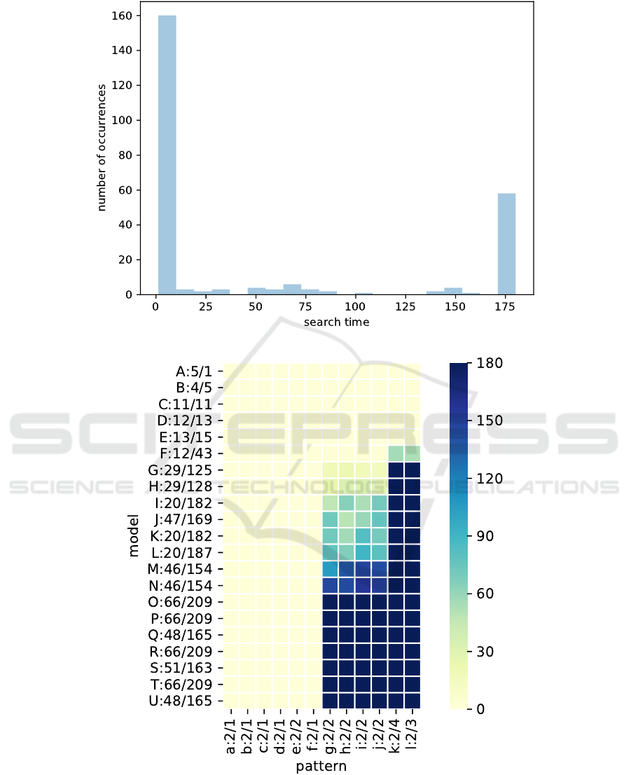
Figure 4: Histogram of search times (in seconds) in the benchmark.
Figure 5: Search times (in seconds) with respect to models and patterns. Models are indicated with an upper-case letter,
patterns with a lower-case letter. Model and pattern names are followed by pairs of numbers e/r: e is the number of entities
and r the number of rules.
relevant for ecologists to (automatically) identify sev-
eral instances of the same interaction pattern (ecologi-
cal processes) in the ecosystem dynamics under study.
Pattern Matching in Discrete Models for Ecosystem Ecology
109

6 CONCLUSION AND
PERSPECTIVES
In this paper, we have presented a method for auto-
matically comparing and assessing similarity between
ecosystems defined as specific kinds of rewriting sys-
tems. We have defined a scoring function that takes
into account not only the number of matching enti-
ties and rules, but also the quality of partial mappings
between the left and right hand sides of rules. The ap-
proach has been successfully applied to the search of
known interaction patterns (i.e., ecological processes)
in models of ecosystems.
The results we have obtained in our benchmark
are promising: we quickly obtain optimal solutions
for the vast majority of the cases studied. For the re-
maining ones, we obtain a solution that is not optimal
in a short time, but we have no assessment of how far
from optimal it is. A possible option to solve this is-
sue could be to add ecological information to assess
the quality of a match (with a relevance score) closer
to the modeler’s expectations. In other words, a big-
ger match is not necessarily a better match. So far,
our method searches for bigger matches. When the
search is interrupted and yields to a sub-optimal so-
lution, a relevance score may help deciding whether
it is already a “good” match or not. In practice, the
matching of entities (here, ecosystemic entities) and
rules (ecological processes) can be guided by adding
additional constraints, such as to:
• enforce the matching/identity between subsets of
entities or rules. For example, if the model al-
lows different categories of rules (each category
possibly having a different semantics), the scor-
ing function could be adapted to take into account
this extension;
• enforce the matching between entities/rules of
the same category (for example match carnivores
among them);
• diminish the importance of some entities/rules
(i.e., set a different weight for each matching up
to forget some, if necessary).
Finally, as a long term perspective, we may use
our method to discover invariant patterns that are not
known in advance, thus increasing the understand-
ing about ecosystem functioning. This could account
for using our concept of similarity to identify match-
ing parts of ecosystems and extract from those the
new patterns. Experiments we have conducted so far
in this direction showed bad performances as search
time becomes prohibitive (as if we would have used
patterns whose sizes are close to the studied models’
sizes). However, sub-optimal patterns may provide
interesting matches (which remains to be studied), or
we may find a way to guide the search with respect to
additional constraints (related to the previous idea of
a relevance score).
ACKNOWLEDGMENT
We would like to thank David Monniaux for his ad-
vise on MAXSAT and PBO solvers, and Daniel Le
Berre who has recommended Sat4j and has been very
helpful concerning its installation and use.
REFERENCES
Agnihotri, K. and Sharma, N. (2015). Developments in eco-
logical modeling based on cellular automata. 6.
Bae, J., Liu, L., Caverlee, J., and Rouse, W. B. (2006). Pro-
cess mining, discovery, and integration using distance
measures. In 2006 IEEE International Conference on
Web Services (ICWS’06), pages 479–488.
Baldan, P., Bocci, M., Cocco, N., and Simeoni, M.
(2013a). Comparing metabolic pathways through
potential fluxes: a selective opening approach. In
BioPPN@Petri Nets.
Baldan, P., Cocco, N., Giummol
`
e, F., and Simeoni, M.
(2013b). Comparing metabolic pathways through re-
actions and potential fluxes. Trans. Petri Nets and
Other Models of Concurrency, 8:1–23.
Baldan, P., Cocco, N., Marin, A., and Simeoni, M. (2010).
Petri nets for modelling metabolic pathways: a survey.
Natural Computing, 9(4):955–989.
Cardelli, L. (2005). Abstract machines of systems biol-
ogy. Transactions on Computational Systems Biology,
3737:145–168.
Danos, V. and Laneve, C. (2004). Formal molecular biol-
ogy. TCS, 325(1):69–110.
Delaplace, F., Di Giusto, C., Giavitto, J., and Klaudel, H.
(2018). Activity networks with delays an application
to toxicity analysis. Fundamenta Informaticae, to ap-
pear.
Dijkman, R., Dumas, M., van Dongen, B., K
¨
a
¨
arik, R., and
Mendling, J. (2011). Similarity of business process
models: Metrics and evaluation. Information Systems,
36(2):498 – 516. Special Issue: Semantic Integration
of Data, Multimedia, and Services.
Ehrenfeucht, A. and Rozenberg, G. (2007). Reaction sys-
tems. Fund. Inform., 75(1-4):263–280.
Euzenat, J. and Shvaiko, P. (2007). Ontology Matching.
Springer-Verlag New York, Inc., Secaucus, NJ, USA.
Fages, F. and Soliman, S. (2008). Formal cell biology
in biocham. In Proceedings of the Formal Meth-
ods for the Design of Computer, Communication, and
Software Systems 8th International Conference on
Formal Methods for Computational Systems Biology,
SFM’08, pages 54–80, Berlin, Heidelberg. Springer-
Verlag.
BIOINFORMATICS 2019 - 10th International Conference on Bioinformatics Models, Methods and Algorithms
110

Gaucherel, C. (2006). Influence of spatial patterns on eco-
logical applications of extremal principles. Ecological
Modelling, 193:531–542.
Gaucherel, C., Boudon, F., Houet, T., Castets, M., and
Godin, C. (2012). Understanding patchy landscape
dynamics: Towards a landscape language. PLoS ONE,
7(9):16.
Gaucherel, C., Houllier, F., AUCLAIR, D., and Houet, T.
(2014). Dynamic Landscape Modelling : The Quest
for a Unifying Theory. Living reviews in landscape
Research, 8(2):5–31.
Gaucherel, C. and Pommereau, F. (2017). Using Petri nets
to identify basins of attraction and tipping points of an
ecosystem. submitted.
Giavitto, J.-L., Malcolm, G., and Michel, O. (2004).
Rewriting systems and the modelling of biological
systems. Comparative and Functional Genomics,
5:95–99.
Grafahrend-Belau, E., Schreiber, F., Heiner, M., Sackmann,
A., Junker, B. H., Grunwald, S., Speer, A., Winder,
K., and Koch, I. (2008). Modularization of biochem-
ical networks based on classification of Petri net t-
invariants. BMC Bioinformatics, 9(1):90.
Henkel, R., Hoehndorf, R., Kacprowski, T., Kn
¨
upfer, C.,
Liebermeister, W., and Waltemath, D. (2018). Notions
of similarity for systems biology models. Briefings in
Bioinformatics, 19(1):77–88.
Le Berre, D. and Parrain, A. (2010). The Sat4j library, re-
lease 2.2. Journal on Satisfiability, Boolean Modeling
and Computation, 7.
Lotka, A. J. (1925). Elements of physical biology. Williams
& Wilkins Company, Baltimore.
May, R. M. (1972). Will a large complex system be stable?
Nature, 238:413 EP –.
Milo, R., Shen-Orr, S., Itzkovitz, S., Kashtan, N.,
Chklovskii, D., and Alon, U. (2002). Network motifs:
Simple building blocks of complex networks. Science,
298(5594):824–827.
Mooiman, L. (2015). Comparing stories with the use of
Petri nets. Technical report, University of Amsterdam.
Paun, A., Paun, M., Rodr
´
ıguez-Pat
´
on, A., and Sidoroff, M.
(2011). P systems with proteins on membranes: a sur-
vey. Int. Journal of Foundations of Computer Science,
22(1):39–53.
PB16 (2016). Pseudo-Boolean competition 2016. http:
//www.cril.univ-artois.fr/PB16. Satellite event
of SAT’16.
Roussel, O. and Manquinho, V. (2012). Input/output
format and solver requirements for the competi-
tions of pseudo-Boolean solvers. http://www.cril.
univ-artois.fr/PB12/format.pdf.
Sangiorgi, D. (2011). Introduction to Bisimulation and
Coinduction. Cambridge University Press, New York,
NY, USA.
SymPy development team (2016). SymPy. http://www.
sympy.org.
Terese (2003). Term Rewriting Systems, volume 55 of Cam-
bridge Tracts in Theoretical Computer Science. Cam-
bridge University Press.
Thomas, R. (1973). Boolean formalisation of genetic con-
trol circuits. Journal of theoretical biology, 42:565–
583.
Tversky, A. (1977). Features of similarity. Psychological
Review, 84(4):327–352.
van Glabbeek, R. and Goltz, U. (1989). Equivalence notions
for concurrent systems and refinement of actions. In
Kreczmar, A. and Mirkowska, G., editors, Mathemat-
ical Foundations of Computer Science 1989, pages
237–248, Berlin, Heidelberg. Springer Berlin Heidel-
berg.
Wang, J., He, T., Wen, L., Wu, N., ter Hofstede, A. H. M.,
and Su, J. (2010). A behavioral similarity measure
between labeled Petri nets based on principal transi-
tion sequences. In On the Move to Meaningful Inter-
net Systems: OTM 2010 - Confederated International
Conferences: CoopIS, IS, DOA and ODBASE, Her-
sonissos, Crete, Greece, October 25-29, 2010, Pro-
ceedings, Part I, pages 394–401.
Xiao, L., Zheng, L., Xiao, J., and Huang, Y. (2009). A
graphical query language for querying Petri nets. In
Yang, J., Ginige, A., Mayr, H. C., and Kutsche, R.-
D., editors, Information Systems: Modeling, Develop-
ment, and Integration, pages 514–525, Berlin, Heidel-
berg. Springer Berlin Heidelberg.
Pattern Matching in Discrete Models for Ecosystem Ecology
111
