
Adversarial Alignment of Class Prediction Uncertainties for Domain
Adaptation
Jeroen Manders
1,2
, Twan van Laarhoven
1,3
and Elena Marchiori
1
1
Institute for Computing and Information Science, Radboud University, Nijmegen, The Netherlands
2
TNO, The Netherlands
3
Faculty of Management, Science and Technology, Open University, Heerlen, The Netherlands
Keywords:
Adversarial Learning, Meta-learning.
Abstract:
We consider unsupervised domain adaptation: given labelled examples from a source domain and unlabelled
examples from a related target domain, the goal is to infer the labels of target examples. Under the assumption
that features from pre-trained deep neural networks are transferable across related domains, domain adaptation
reduces to aligning source and target domain at class prediction uncertainty level. We tackle this problem by
introducing a method based on adversarial learning which forces the label uncertainty predictions on the
target domain to be indistinguishable from those on the source domain. Pre-trained deep neural networks are
used to generate deep features having high transferability across related domains. We perform an extensive
experimental analysis of the proposed method over a wide set of publicly available pre-trained deep neural
networks. Results of our experiments on domain adaptation tasks for image classification show that class
prediction uncertainty alignment with features extracted from pre-trained deep neural networks provides an
efficient, robust and effective method for domain adaptation.
1 INTRODUCTION
In unsupervised domain adaptation, labelled exam-
ples from a source domain and unlabelled examples
from a related target domain are given. The goal is to
infer the labels of target examples. A straightforward
approach for tackling this problem is to label target
examples by just applying a deep neural network pre-
trained on data from a related domain. This approach
has been shown to work rather well in practice. The
reason is that deep networks learn feature represen-
tations which reduce domain discrepancy, although
they do not fully eliminate it (Yosinski et al., 2014).
If we assume that features from pre-trained deep neu-
ral networks indeed provide a good representation for
both source and target data, then in order to perform
domain adaptation one needs to align only source and
target label predictions in such representation, so only
at class label level. This paper investigates this novel
setting. We introduce a label alignment method to
force the uncertainty in the predicted labels on the tar-
get domain to be indistinguishable from that on the
source domain. The method is based on the adversar-
ial learning approach: it performs domain alignment
at class label level by learning a representation that is
at the same time discriminative for the labelled source
data yet incapable of discriminating the source and
target at prediction uncertainty level. Specifically, the
proposed method considers the class probabilities of
a label classifier f as input of a domain discrimina-
tor g. The label classifier f is trained to minimize the
standard supervised loss on the source domain while
the domain discriminator g is trained to distinguish
the class probabilities that the label classifier f out-
puts on the source domain from those on the target
domain (see Fig. 1).
A limitation of this method is that it works only
under the assumption that source and target domains
have the same class distribution. This is because the
representation chosen to minimize the discrepancy
between domains depends on the domains class distri-
bution. If they are different, then the discrepancy be-
tween the domains in our representation will be large.
To overcome this limitation, we introduce a tai-
lored loss function to enforce the domains to have
equal class distributions during our training proce-
dure: we incorporate class weights in our loss func-
tion, one for each instance. Class weights of source
examples are fixed and those of the target examples
are updated during optimization of our loss function.
Manders, J., van Laarhoven, T. and Marchiori, E.
Adversarial Alignment of Class Prediction Uncertainties for Domain Adaptation.
DOI: 10.5220/0007519602210231
In Proceedings of the 8th International Conference on Pattern Recognition Applications and Methods (ICPRAM 2019), pages 221-231
ISBN: 978-989-758-351-3
Copyright
c
2019 by SCITEPRESS – Science and Technology Publications, Lda. All rights reserved
221

Interestingly, training with this loss function leads
to an overestimation of the target domain predictions,
which results in an increased loss while stabilizing ac-
curacy. This approach favors robustness, because the
domain discriminator punishes overconfidence on the
source domain, the latter being a sign of overfitting.
We call the resulting domain adaptation method
LAD (Label Alignment with Deep features).
LAD uses deep features extracted from a pre-
trained deep neural network, so no fine tuning of
the feature extractor is needed. As such, LAD is
more efficient than end-to-end deep learning adapta-
tion methods.
Joint efforts from the machine learning research
community resulted in the public availability of dif-
ferent pre-trained deep neural network architectures
for visual classification. These pre-trained models
provide a rich variety of feature extractors. Besides
trying to align label predictions, the other contribu-
tion of this paper is an extensive analysis of the same
method when changing the ‘feature extractor’ part by
exploring a wide set of existing pre-trained deep ar-
chitectures. This choice allows us to understand the
advantage of the approach when dealing with differ-
ent features.
An extensive experimental analysis shows that
LAD achieves consistent improvement in accuracy
across different pre-trained networks. Overall the
method achieves state of the art results on the stan-
dard Office-31 and ImageCLEF-DA datasets, with a
neat improvement over competing baselines on harder
transfer tasks.
The main contributions of this paper can be sum-
marized as follows: 1) a specific setting for the do-
main adaptation problem; 2) a tailored method for
performing domain adaptation in this setting; 3) ex-
tensive analysis of the proposed method when chang-
ing its ‘feature extraction’ part.
2 RELATED WORK
There is a vast literature on domain adaptation (see
for instance the recent surveys (Weiss et al., 2016;
Csurka, 2017)).
Besides the optimization towards better source
domain class predictions, domain adaptation meth-
ods try to achieve domain invariance (Ben-David
et al., 2010). To achieve domain invariance there are
roughly two popular approaches: minimizing some
measure of domain discrepancy and using an adver-
sarial domain discriminator. Below we summarize
several recent methods based on deep neural net-
works.
Deep-CORAL (Sun and Saenko, 2016) aligns cor-
relations of layer activations in deep neural networks.
Deep Transfer Network (DTN) (Zhang et al., 2015)
employs a deep neural network to model and match
both the domains marginal and conditional distri-
butions. A popular measure used to minimize do-
main discrepancy is Maximum Mean Discrepancy
(MMD) (Gretton et al., 2009). This measure is used
in several recent domain adaptation methods. For
instance, DAN (Long et al., 2015) and RTN (Long
et al., 2016b) are end-to-end deep adaptation meth-
ods which use the sum of multiple MMD by match-
ing the feature distributions of multiple layers across
domains.
In adversarial learning a generator tries to fool
a discriminator so that it cannot distinguish be-
tween generated and real examples(Goodfellow et al.,
2014). Current work on adversarial domain adapta-
tion tries to trick a domain discriminator so that it
no longer can distinguish between features originat-
ing from either the source or target domain, which
results in domain invariant features to be trained.
For instance, ReverseGrad (Ganin and Lempit-
sky, 2015; Ganin et al., 2016) enforce the domains
to be indistinguishable by reversing the gradients of
the loss of the domain classifier.
Recently (Tzeng et al., 2017) introduced a uni-
fying framework for adversarial transfer learning,
and proposed a new instance of this framework,
called Adversarial Discriminative Domain Adapta-
tion (ADDA), which combines discriminative mod-
eling, untied weight sharing, and a generative adver-
sarial network loss.
LAD’s alignment at label level is based on ad-
versarial learning. As such, it shares the theoretical
motivation of adversarial learning method for domain
adaptation, as explained e.g. in (Ganin et al., 2016).
Note that the idea of matching the classifier layer
has been used in end-to-end domain adaptation meth-
ods based on deep learning, for instance DAN and
RTN, where both the feature layer and the classifier
layer are aligned simultaneously using either MMD
or adversarial domain discriminator. The main dif-
ference between LAD and these works is the under-
lying scenario: LAD works under the assumption
that domain representations are already reasonably
matched through the use of a pre-trained deep neural
network for feature extraction. Therefore LAD per-
forms alignment only at class label level, by matching
label predictions. While in LAD the domain discrim-
inator takes as input (source and target) predictions of
the label classifier, in all previous adversarial methods
for domain adaptation the domain discriminator takes
as input (source and target) features.
ICPRAM 2019 - 8th International Conference on Pattern Recognition Applications and Methods
222

3 CLASS PREDICTION
UNCERTAINTY ALIGNMENT
We are given a set S of source images and their labels
drawn from a source domain distribution P
S
(x,y), and
a set T of target images without their labels, drawn
from a target distribution P
T
(x,y). Our goal is to learn
a classifier that correctly predicts the labels of T .
3.1 Label Alignment with Deep
Features
The proposed label alignment method shares the the-
oretical motivation of (adversarial learning) methods
for domain adaptation: find a common representa-
tion that reduces the distance between source and tar-
get domain distributions (Ben-David et al., 2007). In
LAD, as in other adversarial adaptation methods, do-
main distance is reduced using a neural network (the
domain discriminator). In LAD the inputs of the net-
work are class probabilities (computed by softmax),
while in other adversarial methods, like Domain-
Adversarial Neural Networks (Ganin et al., 2016), the
input of the network are (deep) features.
The proposed method tries to align source and tar-
get domain at class label level using two models: a
label classifier C(x, θ
C
), and a domain discriminator
D(y,θ
D
). Both of these functions are parameterized
by neural networks, θ
C
and θ
D
. For brevity we will
omit the parameters θ
C
and θ
D
. The label classifier is
trained to minimize the following standard supervised
loss on the source domain S :
L
S
(C) =
1
|S |
∑
(x,y)∈S
`(C(x),y), (1)
where `(p,y) = −
∑
j
y
j
log(p
j
) is the cross-entropy
loss, and x denotes the vector of features generated
using a pre-trained deep neural network.
The domain discriminator is trained to distinguish
the uncertainty of the predictions that C makes on the
source domain from the uncertainty of the predictions
on the target domain T . This is again a standard su-
pervised problem, predicting d = 1 for the source and
d = 0 for the target, given the output C(x) of the label
classifier. The loss is
L
D
(C,D) =
1
|S |
∑
(x,y)∈S
`(D(C(x)),1)
+
1
|T |
∑
x∈T
`(D(C(x)),0). (2)
We want the label classifier to ‘fool’ the domain
discriminator. This can be achieved by training it
to make the predictions on the two domains indis-
tinguishable. That means that we maximize L
D
with
respect to C. The resulting optimization problem is
therefore
min
C
max
D
L
S
(C) − L
D
(C,D). (3)
3.1.1 Class Weighted Loss Function
Since here we adversarially train a domain invariant
label classifier on the level of predictions, it is nec-
essary that the label distribution of both domains is
the same, otherwise predictions towards certain labels
could be based on possible differences between label
occurrences in both domains.
This would have a negative effect and prevent do-
main alignment. Formally, let c
S
(y) = |{(x
0
,y
0
) ∈
S | y = y
0
}|/|S | be the fraction of source instances
that have label y, and similarly let c
T
(y) be the (un-
known) fraction of target instances with label y under
the true labeling. Then if c
S
(y) 6= c
T
(y) and the la-
bel classifier C makes perfect predictions, the domain
discriminator is able to distinguish the two domains,
based purely on the different conditional probabilities
P(y|d).
To overcome this problem we will switch to
weighted loss functions,
L
S
(C) =
1
|S |
∑
(x,y)∈S
w
S
(x,y)`(C(x),y), (4)
L
D
(C,D) =
1
|S |
∑
(x,y)∈S
w
S
(x,y)`(D(C(x)),1)
+
1
|T |
∑
x∈T
w
T
(x)`(D(C(x)),0).
(5)
Where the weights for the source domain are
w
S
(x,y) =
max
y
0
c
S
(y
0
)
c
S
(y)
. (6)
For the target domain we do not know the true labels,
so instead we use the predicted (pseudo)labels ˜y(x) =
argmax
i
C(x)
i
. So the weights are
w
T
(x) =
max
y
0
˜c
T
(y
0
)
˜c
T
( ˜y(x))
, (7)
where
˜c
T
(y) = |{x
0
∈ T | y = ˜y(x
0
)}|/|T |.
With the weighted loss, the domain discriminator
cannot use the difference in conditional probability
of the class given the domain, since all classes occur
with the same total weight in both domains.
Adversarial Alignment of Class Prediction Uncertainties for Domain Adaptation
223

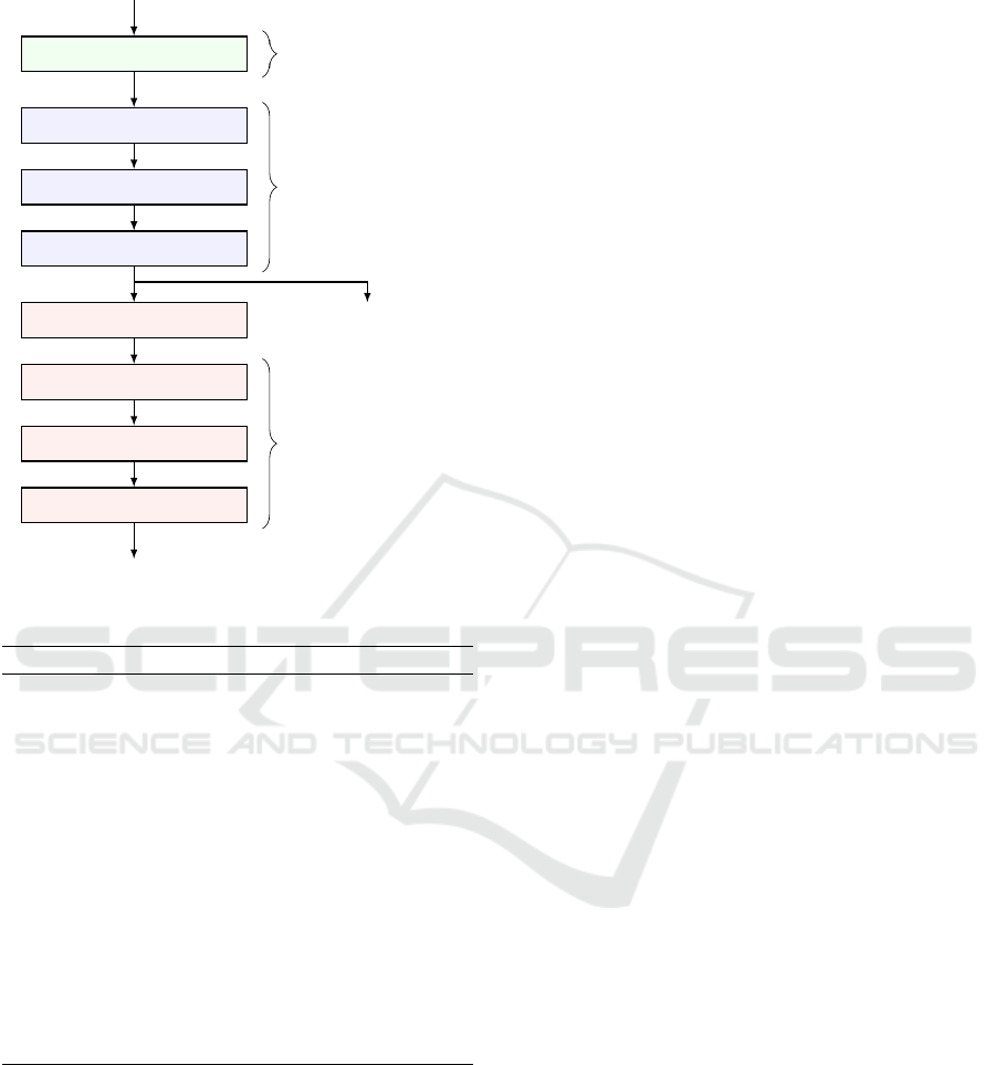
3.2 Architecture
The overall LAD architecture used in our experiments
is shown in Fig. 1. It consists of three parts: feature
extractor, label classifier and domain discriminator.
3.2.1 Feature Extractor
We use a deep neural network pre-trained on the Im-
ageNet dataset (Russakovsky et al., 2015). The last
label prediction layer of a pre-trained network is omit-
ted and features are extracted from the second to last
layer, as this is presumably the layer with the lowest
maximum mean discrepancy (Tzeng et al., 2014).
To generate robust features, we use a form of data
augmentation, where different crops and flips of each
image are passed through the network, and the fea-
tures are averaged.
In particular, for each image, its features are cal-
culated as follows. First, we resize the input image
to the input size of the network plus 64 pixels (for
example, for ResNet50, which expects a 224 × 224
input, we resize the image to 288 × 288 pixels). From
this resized image we take 9 crops spaced of 32 pixels
apart. This is repeated for the horizontally flipped in-
put image, resulting in 18 different image crops. For
each image, crop features are extracted from the pre-
trained network. The final features of the input image
are the averaged features of its 18 crops.
3.2.2 Label Classifier
We consider a label classifier consisting of two dense
(fully connected) layers of size 1024 with ReLu acti-
vation and 0.5 dropout (Srivastava et al., 2014), fol-
lowed by a dense layer with softmax activation for
label predictions.
3.2.3 Domain Discriminator
The considered domain discriminator has the same
structure as the label classifier, but without dropout
layers. The domain discriminator is placed after the
softmax layer of the label classifier, and behind a
gradient reversal layer (Ganin and Lempitsky, 2015;
Ganin et al., 2016) which acts as an identity function
on forward passes through the network, and reverses
the gradient on backward passes. This ensures that
we can use the gradient of L
D
to simultaneously max-
imize with respect to f and minimize with respect to
g in our optimization problem (3).
3.3 Training
All training is done with minibatch Stochastic Gradi-
ent Descent (SGD) with Nesterov momentum. Both
the label and domain loss is calculated with categor-
ical cross-entropy. For training, we assume that we
already extracted the features from a pre-trained deep
neural network. The training of LAD is different from
that of normal feedforward neural networks due to
having two instead of one loss function. Each training
step we draw a minibatch from both domains with-
out replacement, append the domain identifier and,
for the source domain, the class labels. With these
inputs, training proceeds as follows: first, the source
domain batch is used to train the label classifier, then
the source and domain batches are concatenated and
together are used to train the domain discriminator.
We call one pass through the source domain an epoch.
The weights w
T
for the target domain are recom-
puted once per epoch. In the first epoch we set the
weights to 1.
The complete training approach is displayed in
Algorithm 1.
A technical concern of this training procedure is
that as the labels for target domain data are unknown,
in the proposed method, the weights for each target
domain instance are estimated based on the predicted
labels, and then updated iteratively epoch by epoch.
However, there is no guarantee that the iterative pro-
cedure is able to find an optimal solution for w
T
. That
means the estimation of w
T
may become worse and
worse. Nevertheless, under the assumption that fea-
tures extracted from the pre-trained deep neural net-
work are well transferable, and that source and target
domains are related, this phenomenon should not hap-
pen. This is indeed the case in practice, as substanti-
ated by results of our extensive empirical analysis.
4 EXPERIMENTS
We conduct extensive experiments on 12 adaptation
tasks from two real-life benchmark datasets. Datasets,
experimental setup and methods used in our compar-
ative analysis are described in detail below.
4.1 Datasets
We consider two benchmark datasets: Office-31
(Saenko et al., 2010) and imageCLEF-DA
1
.
The Office-31 dataset for visual domain adapta-
tion consists of three domains with images in 31 cat-
egories. The Amazon (A) domain with 2817 images
1
http://imageclef.org/2014/adaptation
ICPRAM 2019 - 8th International Conference on Pattern Recognition Applications and Methods
224
Input
Pre-trained DNN
Dense 1024, ReLu, Dropout
Dense 1024, ReLu, Dropout
Dense, Softmax
Class label
Gradient Reversal Layer
Dense 1024, ReLu
Dense 1024, ReLu
Dense, Softmax
Domain label
Feature extractor
Label classifier
Domain discriminator
Figure 1: LAD Architecture.
Algorithm 1: LAD.
Data: S = labeled source data, T = unlabeled tar-
get data
Result: Y = predicted labels for target domain
w
S
(x,y) ←
max
y
0
c
S
(y
0
)
/c
S
(y) for each (x,y) ∈ S
w
T
(x) ← 1 for each x ∈ T
for epoch ← 1,2, . . . , n
epochs
do
while available batches in S do
S
batch
← take batch from S
T
batch
← take batch from T
Perform a step of SGD on L
S
(C)
Perform a step of SGD on L
D
(C,D)
end while
Y ← ˜y(T )
w
T
(x) ←
max
y
0
c
T
(y
0
)
/ ˜c
T
((x)) for each x ∈ T
end for
consists of images taken from Amazon.com product
pages. The DSLR (D) and Webcam (W) domains,
with respectively 498 and 795 images, consist of im-
ages taken with either a digital SLR or web camera
of the products in different environments. The im-
ages in each domain are unbalanced across the 31
categories, therefore we will use our data balancing
method. We report results on all possible domain
combinations A→D, A→W, D→A, D→W, W→A,
and W→D which is a good combination of difficult
and easier domain adaptation tasks.
The imageCLEF-DA dataset is a benchmark
dataset for ImageCLEF 2014 domain adaptation chal-
lenge and consists of 12 common categories shared by
three public datasets which are seen as different do-
mains: Caltech-256 (C), ImageNet ILSVRC 2012 (I),
and Pascal VOC 2012 (P). This dataset is balanced,
with 50 images for each of the 12 categories for a to-
tal of 600 images per domain, making a good addi-
tion to the Office-31 dataset. Since for each transfer
task the source is balanced, we omit our own balanc-
ing method when using this dataset. We report results
on all domain combinations: C→I, C→P, I→C, I→P,
P→C, P→I.
4.2 Experimental Setup
LAD is implemented on the Tensorflow (Abadi et al.,
2015) framework via the Keras (Chollet et al., 2015)
interface. The network and training parameters are
kept similar across all pre-trained architectures and
domain adaptation tasks of both datasets. Specifically,
we use stochastic gradient descent with a learning rate
of 0.001 and Nesterov momentum of 0.9, a batch size
of 32. All of these parameter settings are considered
default settings. In all our experiments we train each
model for n
epochs
= 1000 epochs. For each transfer
task we run LAD 10 times and report the average la-
bel classification accuracy and standard deviation.
All algorithms are assessed in a fully transductive
setup where all unlabeled target instances are used
during training for predicting their labels. Labeled in-
stances of the first domain are used as the source and
unlabeled instances of the second domain as the tar-
get. We evaluate the accuracy on the target domain as
the percentage of correctly labeled target instances.
In order to assess LAD’s transfer capability, we
consider a baseline variant, obtained by omitting the
domain discriminator from LAD, and trained on the
source data (no adaptation). For instance, Base-
line(DenseNet201) denotes the baseline variant with
the pre-trained DenseNet201 network as the feature
extractor. Network and training parameters are kept
the same as those of LAD across all tasks, besides
training for only 100 epochs which is roughly chosen
as optimal before overfitting becomes a problem.
In all experiments, we did not perform hyperpa-
rameter optimization, but just used default settings of
Keras.
5 RESULTS
In order to assess comparatively the performance of
LAD across different pre-trained architectures, we
Adversarial Alignment of Class Prediction Uncertainties for Domain Adaptation
225

conduct extensive experiments on the following pre-
trained architectures publicly available at Keras: Mo-
bileNet (Howard et al., 2017), VGG16 (Simonyan
and Zisserman, 2014), VGG19 (Simonyan and Zis-
serman, 2014), DenseNet (Huang et al., 2017), In-
ceptionV3 (Szegedy et al., 2016), Xception (Chol-
let, 2016), and InceptionResNetV2 (Szegedy et al.,
2017).
As shown in Table 1, on the Office-31,
LAD(InceptionResNetV2) outperforms the other
variants with an average accuracy of 90.7%. Differ-
ences between architectures are very clear when look-
ing at their baseline results where the difference be-
tween the worst and best architecture is around 10%.
The InceptionResNetV2 pre-trained features are so
good and robust that without LAD they already out-
perform current state-of-the-art methods for domain
adaptation based on the ResNet50 architecture.
On the ResNet50 architecture LAD improves on
our baseline (no adaptation) on all tasks. The im-
provement is more evident on the harder tasks A→D,
D→A, A→W, and W→A. In particular, on A→W
more than 13% improvement is achieved (from 76.5
with no adaptation to 89.9 with adaptation).
The increase in target accuracy is larger when us-
ing less powerful architectures. For example, with
MobileNet, on the harder adaptation tasks D→A
and W→A, about 15% increase in target accuracy is
achieved (from 57.2 with no adaptation to 72.1 with
adaptation for D→A, and from 56.5 with no adapta-
tion to 71.3 with adaptation for W→A).
As shown in Table 2, on the ImageClef-DA adap-
tation tasks, the best average accuracy is obtained by
LAD with the Xception architecture, with an average
accuracy of 89.68%. Notably, on the C→I adaptation
task, using InceptionResNetV2 LAD gains about 11%
target accuracy over the Baseline (from 80.3 with no
adaptation to 91.5 with adaptation).
ImageCLEF-DA results of LAD based on
ResNet50 show that the best improvement over the
Baseline (no adaptation) is obtained on harder tasks.
For instance, on the C→I task (from 80.9 with no
adaptation to 88.5 with adaptation).
LAD consistently performs well on features from
pre-trained deep neural networks with different archi-
tectures.
Overall, results indicate that more recent pre-
trained models achieve very good performance and
that LAD consistently improves on the baselines.
These results provide further experimental evidence
that deep networks learn feature representations
which reduce domain discrepancy, but do not fully
eliminate it, even for architectures achieving excellent
performance, like InceptionResNetV2.
6 COMPARISON WITH
END-TO-END DEEP LEARNING
METHODS
To assess how results of LAD compare with the state-
of-the-art, we report published results of the following
end-to-end deep learning methods for domain adapta-
tion that fine-tune a ResNet50 model pre-trained on
ImageNet: Deep Domain Confusion (DDC) (Tzeng
et al., 2014), Deep Adaptation Network (DAN) (Long
et al., 2015), Residual Transfer Network (RTN) (Long
et al., 2016b), Adversarial Discriminative Domain
Adaptation (ADDA) (Tzeng et al., 2017), Reverse
Gradient (RevGrad) (Ganin and Lempitsky, 2015).
Although all experiments were conducted under
the same transductive setup, results should be inter-
preted with care. There are various differences be-
tween the considered algorithms. For instance, end-
to-end training of a pre-trained deep architecture ver-
sus using the pre-trained architecture to extract fea-
tures, or hyper-parameters tuning vs using default set-
tings.
Overall, results indicate state of the art perfor-
mance of LAD, comparable or better than that of end-
to-end deep adaptation methods.
7 DISCUSSION
7.1 Effectiveness with Shallower
Pre-trained Deep Models
LAD depends on the quality of pseudo labels for com-
puting weights of target instances and for the model
construction. A natural concern is: What if target
classification accuracy is too low? Will the alignment
of classifier predictions still be effective? To inves-
tigate this issue, we consider the shallower network
AlexNet as feature extractor for the Office-31 dataset.
Since this model is not available in Keras, we used
deep features from the 7th layer provided by (Tom-
masi and Tuytelaars, 2014). Table 5 shows results.
When using the less deep AlexNet architecture LAD
still improves on our baseline (no adaptation) on all
tasks. Also in this case, adaptation proves to be ef-
fective on harder tasks. For instance on W→A our
baseline obtains 46.1 accuracy, while with adaptation
54.8 accuracy is achieved.
ICPRAM 2019 - 8th International Conference on Pattern Recognition Applications and Methods
226
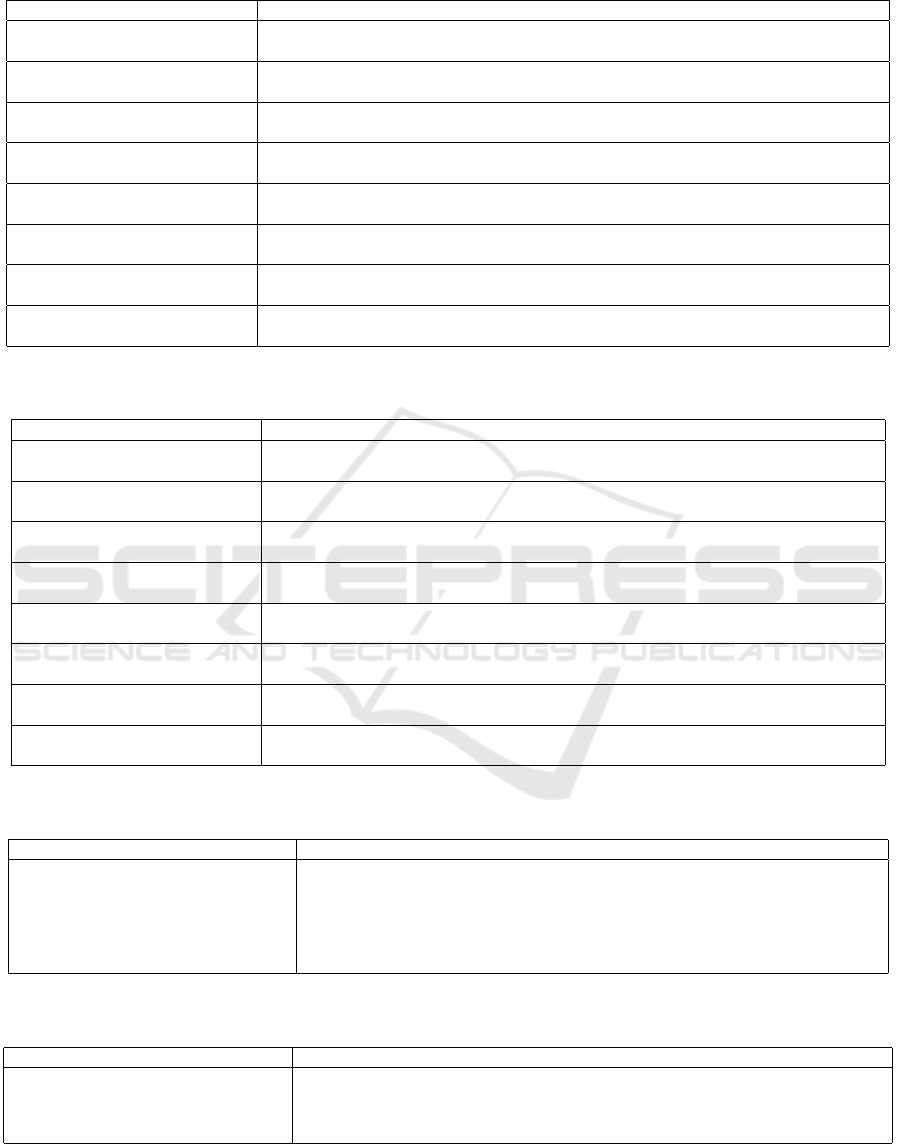
Table 1: Baseline and LAD average accuracy (with standard deviations) over 10 runs on the Office-31 dataset for different
network architectures.
Method A → D A → W D → A D → W W → A W → D avg
Baseline(MobileNet) 74.5±1.5 73.5±0.6 57.2±0.6 97.8±0.2 56.5±0.6 99.4±0.2 76.5%
LAD(MobileNet) 82.2±1.8 89.3±2.5 72.1±0.5 98.9±0.1 71.3±3.2 99.8±0.1 85.6%
Baseline(VGG16) 76.5±1.1 73.7±1.2 61.9±0.6 96.6±0.3 60.4±0.6 99.7±0.1 78.1%
LAD(VGG16) 85.3±2.0 87.9±1.5 69.9±0.8 97.3±0.2 70.1±0.6 99.7±0.1 85.0%
Baseline(VGG19) 76.1±0.8 72.9±1.1 63.4±0.6 97.4±0.4 62.9±1.0 99.8±0.1 78.8%
LAD(VGG19) 83.9±1.8 87.7±0.7 71.0±0.8 98.2±0.3 71.5±0.8 99.9±0.1 85.4%
Baseline(ResNet50) 81.0±0.6 76.5±0.9 64.8±0.8 97.5±0.2 63.6±1.0 99.7±0.2 80.5%
LAD(ResNet50) 90.6±1.2 90.0±0.7 74.0±0.6 98.0±0.1 75.3±1.4 99.8±0.2 87.9%
Baseline(DenseNet201) 85.3±0.8 82.3±1.2 68.5±0.6 98.0±0.2 67.7±0.5 99.9±0.1 83.6%
LAD(DenseNet201) 93.1±0.8 94.7±0.9 77.2±0.8 98.6±0.1 77.7±0.7 99.9±0.1 90.2%
Baseline(InceptionV3) 85.9±0.8 82.4±0.7 72.8±0.4 97.5±0.4 72.8±0.3 99.0±0.3 85.1%
LAD(InceptionV3) 91.2±0.7 88.6±0.5 76.9±0.5 98.3±0.2 76.9±0.8 99.3±0.2 88.5%
Baseline(Xception) 85.2±0.7 83.9±0.7 72.1±0.4 97.0±0.2 71.9±0.5 99.7±0.1 85.0%
LAD(Xception) 91.0±1.5 92.9±0.5 78.6±0.3 98.1±0.1 78.1±0.8 100.0±0.1 89.8%
Baseline(InceptionResNetV2) 90.2±0.7 89.3±0.6 74.9±0.5 97.3±0.2 75.5±0.3 99.6±0.2 87.8%
LAD(InceptionResNetV2) 93.7±0.8 95.3±0.3 78.8±0.5 98.3±0.1 78.5±0.5 99.6±0.1 90.7%
Table 2: Baseline and LAD average accuracy (with standard deviations) over 10 runs on the ImageCLEF-DA dataset for
different network architectures.
Method C → I C → P I → C I → P P → C P → I avg
Baseline(MobileNet) 77.9±0.3 65.2±0.8 89.8±0.7 74.6±0.4 91.2±0.8 84.9±0.8 80.6%
LAD(MobileNet) 87.9±0.7 73.9±0.7 94.6±0.4 75.2±0.5 94.0±0.3 88.3±0.7 85.6%
Baseline(VGG16) 83.2±0.7 70.7±0.5 91.9±0.5 76.5±0.5 91.5±0.6 86.0±0.8 83.3%
LAD(VGG16) 89.6±0.5 76.7±0.8 94.3±0.3 76.2±0.8 94.4±0.4 88.8±0.9 86.7%
Baseline(VGG19) 84.7±0.7 70.9±0.4 92.0±0.3 76.6±0.4 91.6±0.5 85.8±0.7 83.6%
LAD(VGG19) 89.0±0.7 74.5±0.5 94.8±0.3 77.3±0.6 94.3±0.3 90.2±1.0 86.7%
Baseline(ResNet50) 80.9±1.3 68.0±1.0 92.2±0.5 76.1±0.4 91.8±0.5 88.4±0.8 82.9%
LAD(ResNet50) 88.5±1.0 74.0±1.0 95.2±0.4 76.8±0.7 94.1±0.2 90.6±0.6 86.5%
Baseline(DenseNet201) 87.7±0.7 71.6±0.6 93.6±0.4 78.3±0.4 94.3±0.5 90.8±0.8 86.1%
LAD(DenseNet201) 93.0±0.4 78.3±1.0 97.5±0.3 79.1±0.3 95.7±0.4 93.2±0.4 89.5%
Baseline(InceptionV3) 83.1±1.2 66.1±0.8 94.3±0.5 77.8±0.5 93.9±0.4 90.8±0.9 84.3%
LAD(InceptionV3) 92.8±0.3 75.9±0.9 95.9±0.3 78.3±0.5 95.8±0.3 94.2±0.5 88.8%
Baseline(Xception) 85.2±0.8 69.9±0.5 94.7±0.5 79.3±0.5 92.8±1.1 90.8±0.6 85.5%
LAD(Xception) 94.2±0.4 77.7±1.1 96.8±0.4 80.1±0.5 96.6±0.3 92.6±0.6 89.7%
Baseline(InceptionResNetV2) 80.3±0.9 67.8±0.9 90.3±1.9 79.3±0.5 88.4±0.9 89.7±0.8 82.6%
LAD(InceptionResNetV2) 91.5±0.7 75.9±0.9 97.2±0.3 80.6±0.5 95.0±0.3 92.3±1.2 88.7%
Table 3: Average accuracy (with standard deviations) on adaptation tasks from the Office-31 dataset. All methods considered
use a ResNet50 model.
Method A → D A → W D → A D → W W → A W → D avg
DDC (Tzeng et al., 2014) 77.5±0.3 75.8±0.2 67.4±0.4 95.0±0.2 64.0±0.5 98.2±0.1 79.7%
DAN (Long et al., 2015) 78.4±0.2 83.8±0.4 66.7±0. 96.8±0.2 62.7±0.2 99.5±0.1 81.3%
RTN (Long et al., 2016b) 71.0±0.2 73.3±0.2 50.5±0.3 96.8±0.2 51.0±0.1 99.6±0.1 73.7%
RevGrad (Ganin and Lempitsky, 2015) 72.3±0.3 73.0±0.5 52.4±0.4 96.4±0.3 50.4±0.5 99.2±0.3 74.1%
ADDA (Tzeng et al., 2017) 77.8±0.3 86.2±0.5 69.5±0.4 96.2±0.3 68.9±0.5 98.4±0.3 82.9%
LAD 90.6±1.2 89.9±0.7 74.0±0.6 98.0±0.1 75.3±1.4 99.8±0.2 87.9%
Table 4: Average accuracy (with standard deviations) for various methods on the ImageCLEF-DA dataset, obtained with the
ResNet50 architecture.
Method I → P P → I I → C C → I C → P P → C avg
DAN (Long et al., 2015) 75.0±0.4 86.2±0.2 93.3±0.2 84.1±0.4 69.8±0.4 91.3±0.4 83.3%
RTN (Long et al., 2016a) 75.6±0.3 86.8±0.1 95.3±0.1 86.9±0.3 72.7±0.3 92.2±0.4 84.9%
RevGrad (Ganin and Lempitsky, 2015) 75.0±0.6 86.0±0.3 96.2±0.4 87.0±0.5 74.3±0.5 91.5±0.6 85.0%
LAD 76.8±0.7 90.6±0.6 95.2±0.3 88.5±1.0 74.0±1.0 94.1±0.2 86.5%
Adversarial Alignment of Class Prediction Uncertainties for Domain Adaptation
227
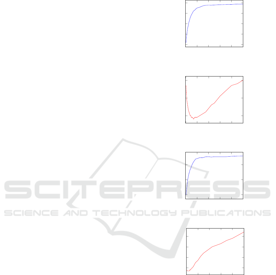
7.2 Robustness to the Choice of the
Number of Epochs
Looking at the learning curves in Fig. 2, we see that
the target domain classification loss reaches a min-
imum after 50 to 150 epochs, after which it starts
to increase. However, the accuracy continues to in-
crease, and there is no sign of overfitting. Ganin &
Lempitsky (Ganin and Lempitsky, 2015) also report
this finding for their method, but it seems this phe-
nomenon is even more pronounced when aligning do-
mains on the level of predictions instead of features.
Indeed, aligning domains on predictions needs to en-
tail the same level of certainty of predictions for both
source and target domains, which leads to an overes-
timation of the target domain prediction certainty, to
match the certainty on the source domain. This over-
estimation in time results in an increased loss while
stabilizing accuracy: a higher certainty of target pre-
dictions makes it harder to switch predictions to an-
other class label.
Furthermore, while the certainty on the source do-
main leads to overconfidence of the label classifier on
the target domain, the uncertainty about the target do-
main labels has a regularizing effect on the source do-
main. The label classifier cannot become overconfi-
dent on the source domain, because then the source
domain predictions would not look like the initially
uncertain target domain predictions.
The stability of the target domain, together with
the regularizing effect of the label uncertainty on the
source domain makes LAD robust to the choice of the
number of epochs. The algorithm therefore does not
require early stopping.
7.3 Class Weights Importance with
Unbalanced Class Distributions
We have also investigated the importance of the
class weights introduced in our loss function (see
Section 3.1.1), by training the model without using
weights.
On the Office-31 dataset, without class weights
LAD with ResNet50 features achieves an average ac-
curacy of 80.3%, compared to 87.9% when the loss
with class weights is used. The Office-31 dataset has
unbalanced class distributions. In this case the loss
with weights prevents the use of this information, and
LAD obtains better performance.
On the other hand, on ImageCLEF-DA, not us-
ing class weights gives an average accuracy of 87.8%,
compared to 86.5% with weights. This happens be-
cause this dataset is fully class balanced. In that case,
performance does not drop when no weights are used
0 200 400
600
800 1,000
80
82
84
86
88
epochs
accuracy (%)
(a) Office-31 accuracy.
0 200 400
600
800 1,000
0.6
0.7
0.8
epochs
class loss
(b) Office-31 loss.
0 200 400
600
800 1,000
82
84
86
epochs
accuracy (%)
(c) ImageCLEF-DA accuracy.
0 200 400
600
800 1,000
0.7
0.8
0.9
1
epochs
class loss
(d) ImageCLEF-DA loss.
Figure 2: Target domain classification accuracy and clas-
sification loss when training for up to 1000 epochs. Made
with the ResNet50 architecture.
in the loss, because class distributions are already
fully class balanced.
In general, we can make no assumptions about the
target domain being balanced. In that case, we should
assume that the data is not class balanced, and use the
weighted loss functions, as is done in LAD.
ICPRAM 2019 - 8th International Conference on Pattern Recognition Applications and Methods
228
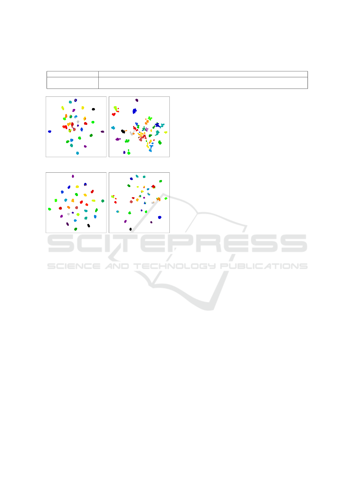
Table 5: Average accuracy (with standard deviations) on adaptation tasks from the Office-31 dataset. LAD uses features
extracted from the 7th layer of the pre-trained AlexNet model.
Method A → D A → W D → A D → W W → A W → D avg
Baseline(DeCAF-fc7) 63.63±1.07 57.26±1.17 47.53±0.75 94.30±0.66 46.15±0.61 98.07±0.42 67.82%
LAD(DeCAF-fc7) 70.78±1.25 65.77±0.56 53.47±0.96 96.78±0.39 54.82±1.18 98.94±0.32 73.43%
(a) Baseline source. (b) Baseline target.
(c) LAD source. (d) LAD target.
Figure 3: t-SNE feature visualization of Baseline and LAD
features on the A→W task from the Office-31 dataset.
ResNet50 is the used pre-trained architecture. Features vi-
sualized from the second dense layer of our architecture
shown in Fig. 1.
7.4 Running Time
LAD does not perform fine-tuning of large pre-trained
architecture weights and therefore is relatively fast
to train. On average over all different transfer tasks
a single epoch as described in algorithm 1 takes
0.4 seconds for Office-31 and 0.2 seconds for the
imageCLEF-DA dataset when trained on a single
Nvidia GeForce GTX 1070.
7.5 Visualization of Deep Features
To get more insight into the feature representation
learned with LAD, we compare t-SNE (Maaten and
Hinton, 2008) feature visualizations of LAD features
with those of Baseline on the ResNet50 architecture.
For better comparability, we visualize features on the
difficult A→W adaptation task. Visualized features
are from the second dense layer (see Fig. 1). Fig. 3
indicates that LAD features are better and more do-
main invariant than those of the baseline, since the
31 classes of the Office-31 dataset are better distin-
guishable and the features from both domains are bet-
ter mapped on each other.
8 CONCLUSION
In this paper we introduced domain alignment at pre-
diction uncertainty level, to be used with features ex-
tracted from pre-trained deep neural networks. We
demonstrated effectiveness, efficiency, and robust-
ness through extensive experiments with diverse pre-
trained architectures and unsupervised domain adap-
tation tasks for image classification.
In our experimental analysis, we did not per-
form hyperparameter optimization, but just used de-
fault settings of Keras. It is interesting to investigate
whether LAD performance could be further improved
by applying procedures for tuning hyperparameters in
a transfer learning setting, like (Zhong et al., 2010).
We have shown that training with our tailored loss
function favors robustness, because the domain dis-
criminator punishes overconfidence on the source do-
main, the latter being a sign of overfitting. It will be
interesting to investigate whether a similar technique
can also be used to prevent overfitting in other set-
tings, such as supervised learning.
A limitation and intrinsic characteristic of LAD is
that it does not directly align source and target fea-
tures, it does alignment only through the uncertainty
of predictions. This is a direct consequence of the
domain adaptation scenario investigated here. As a
consequence, LAD is sensitive to the choice of the
features. Although the results of our experiments
showed that in practice LAD works well across fea-
tures from various pre-trained deep neural networks,
its underlying assumption is the existence (and avail-
ability) of transferable (deep) features. On the other
hand, domain alignment at the feature level as per-
formed by previous domain adaptation methods, no-
tably RevGrad, does not rely on this assumption and
is therefore of more general applicability.
Nevertheless, our method for prediction uncer-
tainty alignment can be applied to any feature repre-
sentation that is good for source and target, so it is not
limited to pre-trained deep neural networks as feature
extractors. It will be interesting in future work to ex-
plore the utility of the method when used on the top of
Adversarial Alignment of Class Prediction Uncertainties for Domain Adaptation
229

domain adaptation methods based on feature transfor-
mation, like (Fernando et al., 2013; Sun et al., 2016).
REFERENCES
Abadi, M., Agarwal, A., Barham, P., Brevdo, E., Chen, Z.,
Citro, C., Corrado, G. S., Davis, A., Dean, J., Devin,
M., Ghemawat, S., Goodfellow, I., Harp, A., Irving,
G., Isard, M., Jia, Y., Jozefowicz, R., Kaiser, L., Kud-
lur, M., Levenberg, J., Man
´
e, D., Monga, R., Moore,
S., Murray, D., Olah, C., Schuster, M., Shlens, J.,
Steiner, B., Sutskever, I., Talwar, K., Tucker, P., Van-
houcke, V., Vasudevan, V., Vi
´
egas, F., Vinyals, O.,
Warden, P., Wattenberg, M., Wicke, M., Yu, Y., and
Zheng, X. (2015). TensorFlow: Large-scale machine
learning on heterogeneous systems. Software avail-
able from tensorflow.org.
Ben-David, S., Blitzer, J., Crammer, K., Kulesza, A.,
Pereira, F., and Vaughan, J. W. (2010). A theory of
learning from different domains. Machine learning,
79(1):151–175.
Ben-David, S., Blitzer, J., Crammer, K., and Pereira, F.
(2007). Analysis of representations for domain adap-
tation. In Advances in Neural Information Processing
Systems, pages 137–144.
Chollet, F. (2016). Xception: Deep learning with
depthwise separable convolutions. arXiv preprint
arXiv:1610.02357.
Chollet, F. et al. (2015). Keras. https://github.com/fchollet/
keras.
Csurka, G. (2017). Domain adaptation for visual appli-
cations: A comprehensive survey. arXiv preprint
arXiv:1702.05374.
Fernando, B., Habrard, A., Sebban, M., and Tuytelaars, T.
(2013). Unsupervised visual domain adaptation using
subspace alignment. In Proceedings of the 2013 IEEE
International Conference on Computer Vision, ICCV
’13, pages 2960–2967, Washington, DC, USA. IEEE
Computer Society.
Ganin, Y. and Lempitsky, V. (2015). Unsupervised domain
adaptation by backpropagation. In International Con-
ference on Machine Learning, pages 1180–1189.
Ganin, Y., Ustinova, E., Ajakan, H., Germain, P.,
Larochelle, H., Laviolette, F., Marchand, M., and
Lempitsky, V. (2016). Domain-adversarial training of
neural networks. Journal of Machine Learning Re-
search, 17(59):1–35.
Goodfellow, I., Pouget-Abadie, J., Mirza, M., Xu, B.,
Warde-Farley, D., Ozair, S., Courville, A., and Ben-
gio, Y. (2014). Generative adversarial nets. In Ad-
vances in Neural Information Processing Systems,
pages 2672–2680.
Gretton, A., Smola, A. J., Huang, J., Schmittfull, M., Borg-
wardt, K. M., and Sch
¨
olkopf, B. (2009). Covariate
shift by kernel mean matching. In Joaquin Quinonero-
Candela, Masashi Sugiyama, A. S. N. D. L., editor,
Dataset Shift in Machine Learning, pages 131–160.
MIT press.
Howard, A. G., Zhu, M., Chen, B., Kalenichenko, D.,
Wang, W., Weyand, T., Andreetto, M., and Adam,
H. (2017). Mobilenets: Efficient convolutional neu-
ral networks for mobile vision applications. arXiv
preprint arXiv:1704.04861.
Huang, G., Liu, Z., van der Maaten, L., and Weinberger,
K. Q. (2017). Densely connected convolutional net-
works. In 2017 IEEE Conference on Computer Vision
and Pattern Recognition (CVPR), pages 2261–2269.
Long, M., Cao, Y., Wang, J., and Jordan, M. (2015).
Learning transferable features with deep adaptation
networks. In International Conference on Machine
Learning, pages 97–105.
Long, M., Wang, J., and Jordan, M. I. (2016a). Deep trans-
fer learning with joint adaptation networks. arXiv
preprint arXiv:1605.06636.
Long, M., Zhu, H., Wang, J., and Jordan, M. I. (2016b).
Unsupervised domain adaptation with residual trans-
fer networks. In Advances in Neural Information Pro-
cessing Systems, pages 136–144.
Maaten, L. v. d. and Hinton, G. (2008). Visualizing data
using t-sne. Journal of Machine Learning Research,
9(Nov):2579–2605.
Russakovsky, O., Deng, J., Su, H., Krause, J., Satheesh, S.,
Ma, S., Huang, Z., Karpathy, A., Khosla, A., Bern-
stein, M., et al. (2015). Imagenet large scale visual
recognition challenge. International Journal of Com-
puter Vision, 115(3):211–252.
Saenko, K., Kulis, B., Fritz, M., and Darrell, T. (2010).
Adapting visual category models to new domains.
Computer Vision–ECCV 2010, pages 213–226.
Simonyan, K. and Zisserman, A. (2014). Very deep con-
volutional networks for large-scale image recognition.
arXiv preprint arXiv:1409.1556.
Srivastava, N., Hinton, G. E., Krizhevsky, A., Sutskever, I.,
and Salakhutdinov, R. (2014). Dropout: a simple way
to prevent neural networks from overfitting. Journal
of machine learning research, 15(1):1929–1958.
Sun, B., Feng, J., and Saenko, K. (2016). Return of frus-
tratingly easy domain adaptation. In Thirtieth AAAI
Conference on Artificial Intelligence.
Sun, B. and Saenko, K. (2016). Deep coral: Correla-
tion alignment for deep domain adaptation. In Com-
puter Vision–ECCV 2016 Workshops, pages 443–450.
Springer.
Szegedy, C., Ioffe, S., Vanhoucke, V., and Alemi, A. A.
(2017). Inception-v4, inception-resnet and the impact
of residual connections on learning. In AAAI, pages
4278–4284.
Szegedy, C., Vanhoucke, V., Ioffe, S., Shlens, J., and Wo-
jna, Z. (2016). Rethinking the inception architecture
for computer vision. In Proceedings of the IEEE Con-
ference on Computer Vision and Pattern Recognition,
pages 2818–2826.
Tommasi, T. and Tuytelaars, T. (2014). A testbed for cross-
dataset analysis. In European Conference on Com-
puter Vision, pages 18–31. Springer.
Tzeng, E., Hoffman, J., Saenko, K., and Darrell, T. (2017).
Adversarial discriminative domain adaptation. In
ICPRAM 2019 - 8th International Conference on Pattern Recognition Applications and Methods
230

2017 IEEE Conference on Computer Vision and Pat-
tern Recognition (CVPR), pages 2962–2971.
Tzeng, E., Hoffman, J., Zhang, N., Saenko, K., and Darrell,
T. (2014). Deep domain confusion: Maximizing for
domain invariance. arXiv preprint arXiv:1412.3474.
Weiss, K., Khoshgoftaar, T. M., and Wang, D. (2016). A
survey of transfer learning. Journal of Big Data,
3(1):9.
Yosinski, J., Clune, J., Bengio, Y., and Lipson, H. (2014).
How transferable are features in deep neural net-
works? In Advances in neural information processing
systems, pages 3320–3328.
Zhang, X., Yu, F. X., Chang, S.-F., and Wang, S. (2015).
Deep transfer network: Unsupervised domain adapta-
tion. arXiv preprint arXiv:1503.00591.
Zhong, E., Fan, W., Yang, Q., Verscheure, O., and Ren,
J. (2010). Cross validation framework to choose
amongst models and datasets for transfer learning. In
Joint European Conference on Machine Learning and
Knowledge Discovery in Databases, pages 547–562.
Springer.
Adversarial Alignment of Class Prediction Uncertainties for Domain Adaptation
231
