
Automatic View Selection for Distributed Dimensional Data
Leandro Ordonez-Ante, Gregory Van Seghbroeck, Tim Wauters, Bruno Volckaert and Filip De Turck
Ghent University - imec, IDLab, Department of Information Technology,
Technologiepark-Zwijnaarde 15, Gent, Belgium
Keywords:
Interactive Querying, View Selection, Clustering, Distributed Data, Dimensional Data, Data Warehouse.
Abstract:
Small-to-medium businesses are increasingly relying on big data platforms to run their analytical workloads
in a cost-effective manner, instead of using conventional and costly data warehouse systems. However, the
distributed nature of big data technologies makes it time-consuming to process typical analytical queries,
especially those involving aggregate and join operations, preventing business users from performing efficient
data exploration. In this sense, a workload-driven approach for automatic view selection was devised, aimed
at speeding up analytical queries issued against distributed dimensional data. This paper presents a detailed
description of the proposed approach, along with an extensive evaluation to test its feasibility. Experimental
results shows that the conceived mechanism is able to automatically derive a limited but comprehensive set of
views able to reduce query processing time by up to 89%–98%.
1 INTRODUCTION
Existing enterprise applications often separate busi-
ness intelligence and data warehousing operations—
mostly supported by Online Analytical Process-
ing systems (OLAP)—from day-to-day transaction
processing—a.k.a. Online Transaction Processing
(OLTP) (Plattner, 2013). While OLTP systems rely
mostly on write-optimized stores and highly normal-
ized data models, OLAP technologies work on top of
read-optimized schemas known as dimensional data
models, which leverage on denormalization and data
redundancy to run computationally-intensive queries
typical from decision-support applications (e.g. re-
porting, dashboards, benchmarking, and data visual-
ization), that would result in prohibitively expensive
execution on fully-normalized databases.
Traditional data warehousing systems are expen-
sive and remain largely inaccessible for most of
the existing small-to-medium sized business (SMEs)
(Qushem et al., 2017). However, thanks to the advent
of big data, more and more cost-effective (often open-
source) tools and technologies are made available for
these organizations, enabling them to run analytical
workloads on clusters of commodity hardware instead
of costly data warehouse infrastructure. Yet in such a
distributed setting, some of the common challenges of
conventional data warehousing systems become even
more daunting to deal with: the way data is scattered
and replicated across distributed file systems such
as Hadoop’s HDFS (Shvachko et al., 2010) makes
it computationally expensive and time-consuming
to run Aggregate-Select-Project-Join (ASPJ) queries
which are one of the foundational constructs of OLAP
operations.
For typical data warehousing and related applica-
tions using materialized views is a common method-
ology for speeding up ASPJ-query execution. The
associated overhead of implementing this methodol-
ogy involves computational resources for creating and
maintaining the views, and additional storage capac-
ity for persisting them. In this sense, finding a fair
compromise between the benefits and costs of this
method is regarded by the research community as the
view selection problem.
In this regard, this paper presents an automatic
view selection mechanism based on syntactic analysis
of common analytical workloads, and proves its effec-
tiveness running on top of distributed dimensionally-
modeled datasets. The paper explores the techniques
devised for abstracting feature vectors from query
statements, clustering related queries based on an es-
timation of their pairwise similarity, and deriving a
limited set of materialized views able to answer the
queries grouped under each cluster.
The remainder of this paper is organized as fol-
lows: Section 2 addresses the related work. Section
3 describes the view selection problem and presents
Ordonez-Ante, L., Van Seghbroeck, G., Wauters, T., Volckaert, B. and De Turck, F.
Automatic View Selection for Distributed Dimensional Data.
DOI: 10.5220/0007555700170028
In Proceedings of the 4th International Conference on Internet of Things, Big Data and Security (IoTBDS 2019), pages 17-28
ISBN: 978-989-758-369-8
Copyright
c
2019 by SCITEPRESS – Science and Technology Publications, Lda. All rights reserved
17

an overview of the proposed approach for tackling
it. Section 4 elaborates on the syntactic analysis con-
ducted on analytical workloads, while Section 5 de-
scribes a proof-of-concept implementation of the de-
vised mechanism, along with the experimental setup
and performance results. Finally conclusions and fu-
ture work are addressed in Section 6.
2 RELATED WORK
Extensive research has been conducted around the
view selection problem, as evidenced in several sys-
tematic reviews on the topic such as those by (Thakur
and Gosain, 2011), (Nalini et al., 2012), (Goswami
et al., 2016), (Gosain and Sachdeva, 2017). The re-
view elaborated in (Goswami et al., 2016) groups
existing approaches in three main categories: (i)
heuristic approaches, (ii) randomized algorithmic ap-
proaches, and (iii) data mining approaches.
Heuristic and randomized algorithmic approaches
emerged as an attempt to provide approximate opti-
mal solutions to the NP-Hard problem that view se-
lection entails. Both types of approaches use mul-
tidimensional lattice representations (Serna-Encinas
and Hoyo-Montano, 2007), AND-OR graphs (Sun
and Wang, 2009; Zhang et al., 2009), or multiple
view processing plan (MVPP) graphs (Phuboon-ob
and Auepanwiriyakul, 2007; Derakhshan et al., 2008)
for selecting views for materialization. Issues re-
garding the exponential growth of the lattice structure
when the number of dimensions increases, and the
expensive process of graph generation for large and
complex query workloads, greatly impact the scala-
bility of these approaches and their actual implemen-
tation in consequence (Aouiche et al., 2006; Goswami
et al., 2016).
Unlike previously mentioned approaches, data-
mining based solutions work with much simpler in-
put data structures called representative attribute ma-
trices, which are generated out of query workloads.
These structures then configure a clustering context
out of which candidate view definitions are derived.
In (Aouiche et al., 2006; Aouiche and Darmont, 2009)
candidate views are generated by merging views ar-
ranged in a lattice structure. Since the number of
nodes in this lattice grows exponentially with the
number of views, the procedure for traversing it can
be expensive. Other data mining approaches for
view selection, including the one from (Kumar et al.,
2012), involve browsing across several intermediate
and/or historical results, which is deemed to be a very
costly and unscalable process (Goswami et al., 2016).
More recently, approaches such as (Goswami
et al., 2017) and (Camacho Rodriguez, 2018) explore
the application of materialized views on top of mas-
sive distributed data to speed up big data query pro-
cessing. While the work of Goswami et al. (Goswami
et al., 2017) addresses a solution based on a multi-
objective optimization formulation of the view selec-
tion problem, it assumes as given the set of candi-
date views from which the selection is made. On the
other hand, (Camacho Rodriguez, 2018) elaborates on
the recently enabled support for materialized views in
Apache Hive (Vohra, 2016b), however at the time of
writing there is no indication of any built-in mecha-
nism for supporting view selection with this new fea-
ture.
In view of the above, this paper elaborates on
an automatic mechanism for materialized view se-
lection on top of distributed dimensionally-modeled
data. The mechanism presented in the following sec-
tions relies on syntactic analysis of query workloads
using a representative attribute matrix as input data
structure, assembled as a collection of feature vec-
tors encoding all the clauses of each individual query
in the workload at hand. With this input, a strat-
egy for selecting a limited set of candidate material-
izable views is implemented, comprising the use of
hierarchical clustering along with a custom query dis-
tance function complying with the structure of the
feature vectors, and the estimation of a materializable
score on the resulting clustering configuration, allow-
ing to unambiguously identify materializable groups
of queries.
3 MATERIALIZED VIEW
SELECTION
Before addressing an overview of the proposed ap-
proach, let’s first define the view selection problem.
Definition 1. View Selection Problem. Based on
the definition by Chirkova et al. (Chirkova et al.,
2001): Let R be the set of base relations (compris-
ing fact(s) and dimensions tables), S the available
storage space, Q a workload on R , L the function
for estimating the cost of query processing. The view
selection problem is to find the set of views V (view
configuration) over R whose total size is at most S
and that minimizes L(R , V , Q )
In the context of the view selection approach pro-
posed herein, some assumptions are made for the sys-
tem to identify and materialize candidate views out of
the syntactic analysis of query workloads:
1. The source data collection (D
src
) complies a star
schema data model, i.e. it comprises a fact table
IoTBDS 2019 - 4th International Conference on Internet of Things, Big Data and Security
18
[[2,10,0,...,12,24,8],
[4,12,1,...,15,36,9],
[2,14,0,...,16,28,4],
...
[8,12,2,...,40,44,9]]
D
src
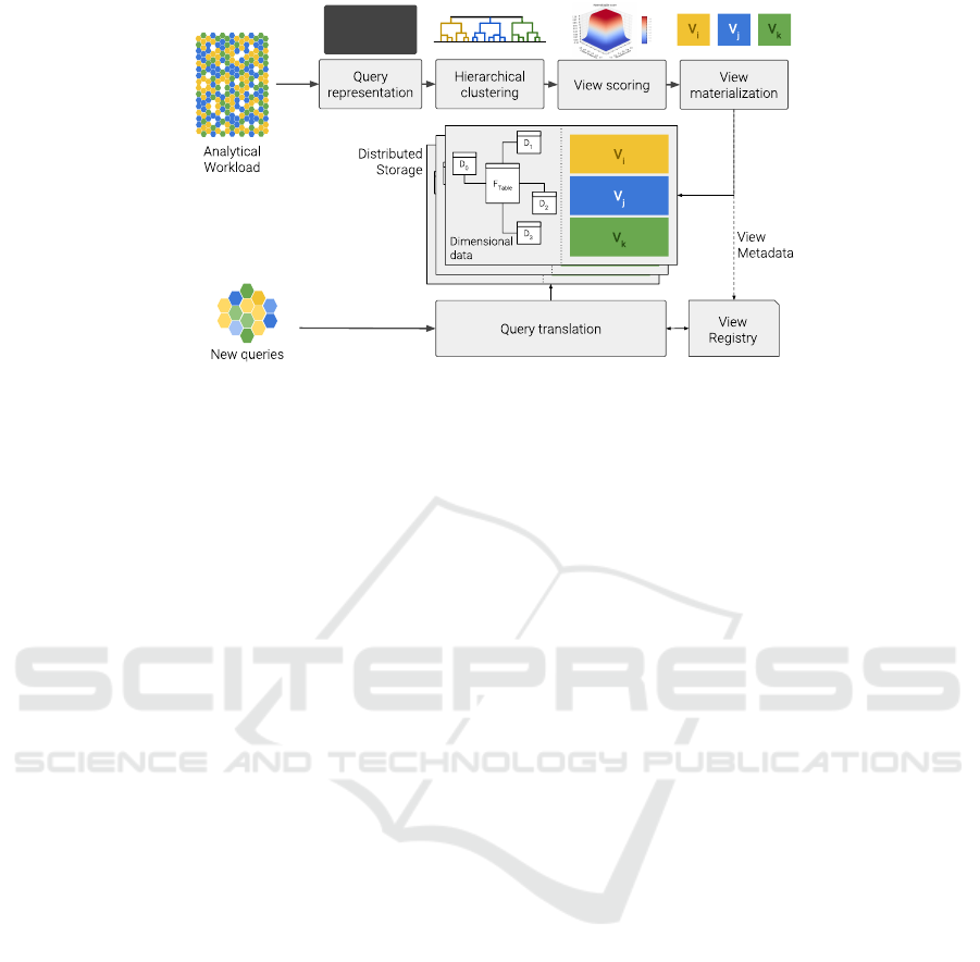
Figure 1: Materialized view selection: architecture overview.
referencing one or more dimension tables.
2. D
src
is temporary immutable. This is a com-
mon scenario in some data warehousing systems,
where analytical data is updated once in a sub-
stantial period of time —e.g. through an ETL pro-
cedure running on top of OLTP databases—, and
queried multiple times during such a period.
3. Statistical information regarding D
src
, such as the
size (row count) of each of the base tables com-
posing the dataset, as well as the cardinality of
the attributes that make up these relations is avail-
able either by querying the metadata kept by the
datastore, or by directly querying the base tables.
4. Latency is favored over view storage cost. This
means that the decision on materializing candi-
date views is driven not by storage restrictions, but
by the gain in query latency.
Figure 1 outlines the main components of the mech-
anism proposed herein to address the stated view se-
lection problem. In terms of the definition 1, given
a dimensionally modeled dataset R and a workload
Q , the view selection mechanism starts by translat-
ing the queries in Q into feature vectors represent-
ing the attributes contained in each of the clauses of
an ASPJ-query, i.e. aggregate operation, projection,
join predicates and range predicates. In contrast to
similar query representations such as the one used in
(Aouiche et al., 2006), the method proposed herein
accounts not only for query-attribute usage, but also
for query structure by defining a number of region-
s/segments representative of each of the clauses of a
Select-Project-Join (SPJ) query, i.e. aggregate opera-
tion, select list, join predicates and range predicates.
This way, the devised query representation provides a
more precise specification of the query statements in
Q .
The collection of feature vectors of Q configure
a clustering context C . This context is then fed to a
clustering algorithm able to identify groups of related
queries based on a similarity score computed via a
custom query distance function. Upon running the
clustering job, the resulting clustering configuration
K comprises several groups of queries the algorithm
deemed to be similar. The idea behind building this
clustering configuration is to be able to deduce view
definitions covering the queries arranged under each
cluster. The clustering algorithm might come up with
spurious clusters, i.e. groups of queries that are actu-
ally not that related. To identify those spurious clus-
ters and setting them apart from those clusters whose
corresponding candidate views are worth materializ-
ing, a materializable score is defined, taking into ac-
count a measure of cluster consistency and the cluster
size. Further details on this score and the clustering
procedure are provided later in section 4.2.
Based on the results of the materializable score
computed on the clustering configuration K , a subset
of the candidate views in V , V
mat
, is prescribed to
be materialized. Finally, with the views in place, the
translation of new analytical queries matching said
views is performed.
4 QUERY ANALYSIS
ASPJ-queries allow for summarization returning a
single row result based on multiple rows grouped to-
gether under certain criteria (column projection and
range predicates).
The syntactic analysis this work thrives on, starts
by mining the information contained in the select list
and search conditions clauses, encoding these values
in a feature vector representation that enables further
query processing.
Automatic View Selection for Distributed Dimensional Data
19

4.1 Query Representation
The procedure for obtaining a text-mining-friendly
representation of the queries takes each one of the
SELECT statements from a workload Q and extracts
the aggregate (ag
q
) and projection (p j
q
) elements,
and join ( jn
q
) and range (rg
q
) predicates, resulting
in the following tuple:
q = (ag
q
, p j
q
, jn
q
, rg
q
) (1)
The tuple above is the high-level vector represen-
tation of the queries from Q . Consider for example
the following SELECT statement:
SELECT SUM( lo _ r e ve n u e ) , d_ye ar ,
p_ c a t eg o ry
FROM lin eor der , d w date , pa r t
WHERE lo _ or d er d at e = d_ da t e k ey
AND lo _ pa rt k ey = p_ p a r tk e y
AND d_ y e a r > 2 0 10
GROUP BY d_ye a r , p_ ca t eg o r y
For the query above:
ag
q
= [SUM, lo revenue]
p j
q
= [d year, p category]
jn
q
= [d datekey, p partkey]
rg
q
= [d year]
Each element of the above high-level vector represen-
tation gets mapped to a vector using a binary encoding
function, as described below.
Definition 2. Binary Mapping Function. Let R be a
relation defined as a set of m attributes (a
1
, a
2
, ..., a
m
)
—with a
m
being the primary key of R—, and given
r an arbitrary set of attributes, the binary mapping
of r according to R, denoted by bm
R
(r), is defined as
follows:
bm
R
(r) =
{
b
i
}
, 1 ≤ i ≤ m
b
i
=
(
1, if a
i
∈ r
0, otherwise
(2)
Using the mapping function above, the vector rep-
resentation of each one of the query elements in Eq.1
(designated henceforth as segments), for a dimen-
sional schema comprising one fact table and N dimen-
sion tables, is defined as follows:
ag
q
= [aggOpCode, bm
Fact
(ag
q
)]
pj
q
= [bm
Fact
(p j
q
), bm
Dim1
(p j
q
), ..., bm
DimN
(p j
q
)]
jn
q
= [bm
Dim1
( jn
q
), ..., bm
DimN
( jn
q
)]
rg
q
= [bm
Fact
(rg
q
), bm
Dim1
(rg
q
), ..., bm
DimN
(rg
q
)]
where aggOpCode designates the aggregate operation
using one-hot encoding, namely, COUNT: 00001, SUM:
00010, AVG: 00100, MAX: 01000, MIN: 10000.
A complete feature vector q representing a query
q ∈ Q is set by putting together the above-mentioned
segments, that is:
q = [ag
q
, pj
q
, jn
q
, rg
q
]
Accordingly, considering the SELECT statement in
the example above and the dimensional schema de-
scribed in (O’Neil et al., 2009) which comprises one
fact table and four dimension tables, a complete fea-
ture vector instance (its decimal equivalent for length
and clarity) is shown below:
q = [[2, 8] , [0, 0, 16, 8, 0] , [0, 1, 1, 0] , [0, 0, 16, 0, 0]]
The collection of feature vectors representing the
queries from Q are arranged as a representative at-
tribute matrix, configuring a clustering context C .
4.2 Query Clustering and View
Materialization
The view selection approach documented herein re-
lies on hierarchical clustering (Friedman et al., 2009)
for deriving groupings of similar queries. In contrast
to other well-known clustering methods such as K-
Means or K-medoids, hierarchical clustering analy-
sis does not require the number of clusters upfront
as parameter. Instead, it generates a hierarchical rep-
resentation of the entire clustering context in which
observations and groups of observations are stacked
together from lower to higher levels, according to a
distance measure based on the pairwise dissimilarities
among the observations.
This way, a dissimilarity metric is required to ap-
ply hierarchical clustering analysis on a clustering
context C , along with a linkage criterion which es-
timates the dissimilarity among groups of queries as
a function of the pairwise distance computed between
queries belonging to those groups. In this sense, a
distance function, qDst, is defined in which similar-
ity between two queries is determined to be propor-
tional to the number of attributes they share in a per-
segment and per-relation (fact and dimensions) basis.
Since vectors in C do not lie in an euclidean space, the
Weighted Pair Group Method with Arithmetic Mean
(WPGMA) clustering method is used as linkage cri-
terion, instead of methods such as centroid, median,
or ward (M
¨
ullner, 2011).
Under this set-up, the clustering procedure (de-
tailed in algorithm 1) starts by assigning each query
to its own cluster (see line 1). Then, the pairwise dis-
similarity matrix between these singleton clusters, D,
IoTBDS 2019 - 4th International Conference on Internet of Things, Big Data and Security
20

Algorithm 1: WPGMA clustering procedure.
1: K ← C ; C = {q
0
, q
1
, . . . , q
N
} Initializing clusters (singleton clusters)
2: D ← qDst(q
i
, q
j
) for all q
i
, q
j
∈ K , i 6= j Pairwise dissimilarity matrix
3: L ← [] Output matrix
4: while |K | > 1 do
5: (a, b) ← argmin(D) Get the nearest clusters
6: append [a, b, D [a, b]] to L
7: remove a and b from K
8: create new cluster k ← a ∪ b Merge a and b into one cluster
9: update D: D [k, x] = D [x, k] =
qDst(a,x)+qDst(b,x)
2
for all x ∈ K
10: K ← K ∪ k
11: end while
12: return K , L L: WPGMA dendrogram: ((N − 1) × 3)-matrix
is computed and an empty matrix (L) specifying the
resulting dendrogram is initialized (lines 2-3). From
D, the two most similar (nearest) clusters are merged
into one, and appended to L along with the distance
between them (lines 5-6). Then, the pairwise dissimi-
larity matrix gets updated using the WPGMA method
for computing the distance between the newly formed
cluster and the rest of the currently existing clusters
(eq. 3):
D[(a ∪ b), x] =
qDst(a, x) + qDst(b, x)
2
,
(a, b and x being clusters)
(3)
This procedure is then repeated until there is only
one cluster left. Finally, both the clustering configura-
tion (K ) and the dendrogram matrix (L) are returned
(line 12).
As mentioned earlier, spurious clusters might be
found in the derived clustering configuration. To
avoid further processing of those query groups a score
was defined indicating to what extent it is worth to
materialize the view derived from a particular cluster.
Definition 3. Materializable Cluster. A cluster c
from a clustering configuration K is said to be ma-
terializable if the following conditions are met:
1. Queries in c are highly similar to each other.
2. Queries in c are clearly separated (highly dissim-
ilar) from queries in other clusters.
3. |c| is large enough in proportion to the size of the
workload |Q |.
A cluster meeting the first two conditions is said to
be a consistent cluster, while the third condition pre-
vents singleton and small clusters from being further
processed. Based on the above definition, the materi-
alizable score of a cluster (mat(c) in eq. 4) is com-
puted as the product of two sigmoid functions: one
on the per-cluster silhouette score (S) (Rousseeuw,
1987)—defined below in eq. 5—and the other on the
per-cluster proportions (P).
mat(c) =
1
1 + e
−k(S(c)−s
0
)
1
1 + e
−k(P(c)−p
0
)
(4)
With:
S(c) =
1
|
c
|
∑
q
i
∈c
b(q
i
) − a(q
i
)
max
{
a(q
i
), b(q
i
)
}
, P(c) =
|c|
|Q |
(5)
Where,
• k is a factor that controls the steepness of both of
the sigmoid functions,
• s
0
and p
0
are the midpoints of the silhouette and
cluster-proportion sigmoids respectively,
• a(q
i
) is the average distance between q
i
and all
queries within the same cluster,
• b(q
i
) lowest average distance of q
i
to all queries
in any other clusters.
Upon factoring out the spurious clusters, the next
step is deriving view definitions covering the queries
arranged under each of the materializable clusters
(K
mat
⊆ K ). Algorithm 2 below details the proce-
dure conducted to derive the views V
i
meeting this
containment condition on each of the materializable
clusters. In this procedure, the ASPJ clauses of the
resulting views are defined in terms of the union of
the corresponding attributes from each query in the
cluster (aggregate (ag
q
), projection (p j
q
), join ( jn
q
),
and range (rg
q
) predicates in lines 4-7).
Automatic View Selection for Distributed Dimensional Data
21

Algorithm 2: Procedure for deriving view definitions.
1: Let c be a cluster in K
mat
2: V ← [ag
V
, p j
V
, jn
V
, groupBy
V
] Output view
definition
3: for each query q in c do
4: ag
V
← ag
V
∪ ag
q
5: p j
V
← p j
V
∪ p j
q
∪ rg
q
6: jn
V
← jn
V
∪ jn
q
7: groupBy
V
← groupBy
V
∪ p j
q
∪ rg
q
8: end for
9: return V
5 EVALUATION
5.1 Proof-of-concept Implementation
A bottom-up approach was adopted to test the view
selection mechanism detailed in the previous sections.
In this way, starting from a set of predefined view
definitions, the effectiveness of the proposed mecha-
nism is estimated in terms of its ability for identifying
the same set of views and reconstructing their defi-
nitions, upon analyzing a query workload generated
from query templates fitting the original set of views
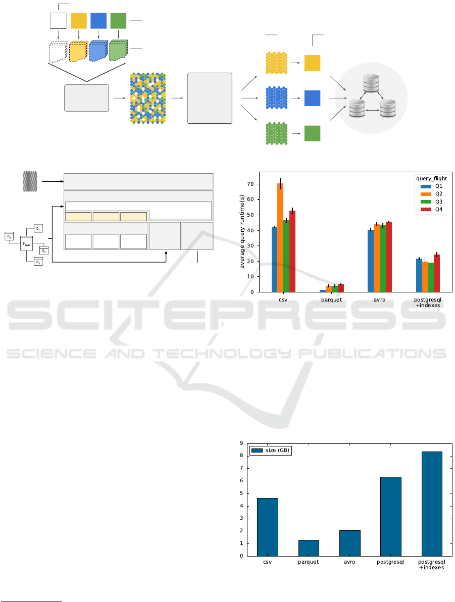
(see Figure 2).
This proof-of-concept implementation leverages
the Star Schema Benchmark (SSB) as baseline
schema and dataset, and therefore both the predefined
views and query templates, as well as the query gener-
ator module were designed and built so they conform
to the data model the SSB embodies.
Thirteen ASPJ-query statements compose the full
query set of the SSB, arranged in four categories/fam-
ilies designated as Query Flights (a detailed definition
of the SSB is available at (O’Neil et al., 2009)). For
this proof-of-concept, three view definitions were de-
rived based on the original SSB query set, and from
each view definition, four query templates were pre-
pared. Additionally, one template per each one of the
13 canonical SSB queries were also composed. With
this set of 25 templates as input, a module that gener-
ates random instances of runnable queries enabled the
creation of query workloads of arbitrary size. Listings
below present the definitions of each one of the men-
tioned views.
Listing 1: Definition of View A.
SELECT sum( lo _ r e ve n u e ) , p_ bra nd1 ,
c_r egi on ,
s_r egi on , d _ ye ar
FROM lin eor der , c ust ome r , dwdate ,
par t , s u p pl ie r
WHERE lo _ cu st k ey = c_ c us tk e y
AND lo _ or d er d at e = d_ da t e k ey
AND lo _ pa rt k ey = p_ p a r tk e y
AND lo _ su pp k ey = s_ s u p pk e y
GROUP BY p_ bra n d1 , c_ reg ion ,
s_r egi on , d _ ye ar
ORDER BY p_ bra n d1 , c_ reg ion ,
s_r egi on , d _ ye ar
Listing 2: Definition of View B.
SELECT sum( lo _ o rd t ot a l p r i ce ) ,
p_ c at eg o ry , c _ city ,
s_cit y , d_ y ea r mo n th n um
FROM lin eor der , c ust ome r , dwdate ,
par t , s u p pl ie r
WHERE lo _ cu st k ey = c_ c us tk e y
AND lo _ or d er d at e = d_ da t e k ey
AND lo _ pa rt k ey = p_ p a r tk e y
AND lo _ su pp k ey = s_ s u p pk e y
GROUP BY p _ ca te g or y , c_cit y , s_ c ity ,
d_ y ea r m o n t h n u m
ORDER BY p _ ca te g or y , c_cit y , s_ c ity ,
d_ y ea r m o n t h n u m
Listing 3: Definition of View C.
SELECT sum( lo _ su p pl y co s t - l o_ ta x ) ,
c_r egi on , p_mfg r ,
s_r egi on , c_ n ati on , d _y ea r
FROM lin eor der , c ust ome r , dwdate ,
par t , s u p pl ie r
WHERE lo _ cu st k ey = c_ c us tk e y
AND lo _ or d er d at e = d_ da t e k ey
AND lo _ pa rt k ey = p_ p a r tk e y
AND lo _ su pp k ey = s_ s u p pk e y
GROUP BY c_ reg i on , p_m f gr , s_re gio n ,
c_n ati on , d _ ye ar
ORDER BY c_ reg i on , p_m f gr , s_re gio n ,
c_n ati on , d _ ye ar
5.2 Definition of the Data Serialization
Format
Since serialization formats determine the way data
structures are turned into bytes and sent over the net-
work, and how said structures are stored on disk, such
formats have a major impact on the response time of
data processing and retrieval operations performed in
a distributed fashion. This is why, prior to evaluat-
ing the performance of the proposed view selection
mechanism, the decision on which serialization for-
mat to use for encoding and storing the SSB datasets
into HDFS needed to be made. Figure 3 outlines the
setup arranged to conduct a benchmark analysis on
three different data serialization formats, one being
a text-based format (CSV) and two binary schema-
driven formats (Parquet (Vohra, 2016c) and Avro
IoTBDS 2019 - 4th International Conference on Internet of Things, Big Data and Security
22
View
Selection
(PoC)
V
A
V
B
V
C
Predefined view
definitions
Query templates
Query
Generator
Workload
V
A
V
B
V
C
D
trg
Materializable
clusters
Reconstructed
views
SSB
SSB-based queries
Distributed storage
Figure 2: Proof-of-concept implementation of the proposed view selection mechanism.
Hadoop
DNode 1 DNode 3DNode 2
Spark SQL
Jupyter Notebook
SSB Workload
PostgreSQL
SSB dataset
(48 million rows)
MongoDB
View registry
CSV AVROPARQUET
SSB storage & querying
Figure 3: Set-up for deciding on the data serialization for-
mat.
(Vohra, 2016a)). By leveraging on the built-in sup-
port Spark SQL provides for these serialization for-
mats, a 48-million-row SSB dataset was encoded into
CSV, Parquet and Avro and stored in HDFS. Then,
the canonical SSB query set (consisting of 13 queries)
was run against each of the encoded datasets, as well
as against a separate dataset placed in a single-node
PostgreSQL
1
database serving as a reference.
Figure 4 shows the results obtained from mea-
suring the average query runtime (over 10 runs) for
each one of the serialization formats. Notice how, in
the mentioned conditions, queries running against the
Parquet-encoded dataset ran up to 10 times faster than
the reference relational database. Also, Parquet was
the only serialization format that managed to outper-
form the average query runtime of PostgreSQL.
Serialization formats also have a significant im-
pact on the size of the encoded data structures. While
for text-based human-readable formats such as CSV
data is stored as-is, binary formats like Parquet and
Avro do apply compression on the data they encode.
Figure 5 shows a comparison between the reported
sizes (in gigabytes) of the SSB dataset for each of the
considered serialization formats. According to these
results Parquet is once again the most efficient serial-
1
PostgreSQL 9.5.8 working with the default configura-
tion and deployed on a VMWare
R
virtual machine as the
ones used for the Hadoop cluster (postgresql.org)
Figure 4: Average query-flight runtime per data serializa-
tion format (SSB SF = 8).
ization format, reaching a compression ratio of 3.6:1
in relation to the uncompressed CSV-encoded dataset,
and 6.5:1 in relation to the PostgreSQL reference
database (including primary key indexes). In conse-
quence, Parquet was the chosen serialization format
for encoding the various datasets involved in the eval-
uation of the proposed view selection approach.
Figure 5: Disk space usage per data serialization format
(SSB SF = 8).
Automatic View Selection for Distributed Dimensional Data
23
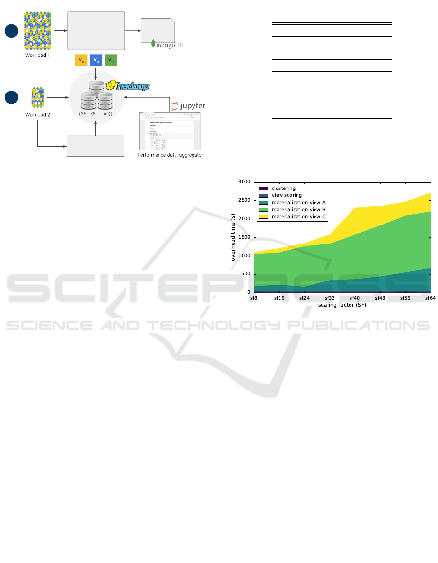
5.3 Experimental Setup
View Selection (PoC)
1
View
Registry
Query translator
2
SSB
Figure 6: View selection experiment set-up.
Figure 6 depicts the arrangement of components
and technologies used for conducting the experimen-
tal evaluation of the proposed view selection ap-
proach. This evaluation comprised two major stages:
(1) Running the view selection implementation on a
400-query workload to the point it materializes
views A, B, and C (defined in section 5.1), while
keeping track of the runtime involved in the proce-
dures of query clustering, view scoring (using the
materializable score defined in section 4.2), and
view creation (i.e. materialization).
(2) Once the views are materialized, run a 100-query
workload against both the base SSB dataset and
the materialized views. In doing the latter, work-
load queries first pass through a translation com-
ponent that gathers the details of the available
materialized views from the view registry (stored
in a MongoBD
2
2.6.10 document database), and
adapts the incoming query statements accord-
ingly.
For all the stages, the performance information
collected from running the tests were aggregated
and visualized using Jupyter notebook
3
. During this
evaluation, workloads were run against eight different
sizes of the SSB dataset, as specified below in table
1. These datasets were stored into a 3-Node Hadoop
4
2.7.3 cluster deployed on 3 VMWare
R
virtual
machines, each one with the following specifications:
Intel
R
Xeon
R
E5645 @2.40GHz CPU, 16GB
RAM, 250GB hard disk.
2
Available at mongodb.com
3
Available at jupyter.org
4
Available at hadoop.apache.org
Table 1: SSB dataset sizes.
Scaling
Factor (SF)
Dataset size
(# rows)
8 48×10
6
16 96×10
6
24 144×10
6
32 192×10
6
40 240×10
6
48 288×10
6
56 336×10
6
64 384×10
6
5.4 Results
5.4.1 View Selection Overhead
Figure 7: View selection runtime per process (|Q | = 400).
Time needed for view materialization grows as the dataset
size increases, while the overhead due to clustering and
view scoring remains invariant.
The overhead of the view selection implementa-
tion was estimated first by running it on a 400-query
workload throughout the considered range of sizes of
the SSB dataset. Results show that, for a fixed-size
workload, the runtime overhead grows nearly propor-
tional to the size of the data collection (See Figure 7),
with a major part of said overhead due to the view ma-
terialization itself. As mentioned before, the proposed
view selection mechanism involves the execution of a
sequence of steps: (1) query clustering, (2) view (or
cluster) scoring, and (3) view materialization. Out
of these only the first two steps have to do with the
syntactical analysis of query sets described through-
out this paper, while the last one refers to the actual
materialization of the derived views in Parquet. Fig-
ure 7 shows the execution times for each one of the
three mentioned steps, including the individual ma-
terialization of each one of the three selected views.
Note how clustering and view scoring amount to only
20 seconds, and remain largely invariant as the dataset
size grows larger. Nonetheless, it is worth mentioning
IoTBDS 2019 - 4th International Conference on Internet of Things, Big Data and Security
24
that the behaviour evidenced in Figure 7 for the ma-
terialization step cannot be assumed the same for any
arbitrary set of views, since this part of the runtime
overhead depends not only on the size of the dataset,
but also on factors such as view size, the join pred-
icates in the view definition, and —given that views
are placed in a distributed file system— also the la-
tency of the network.
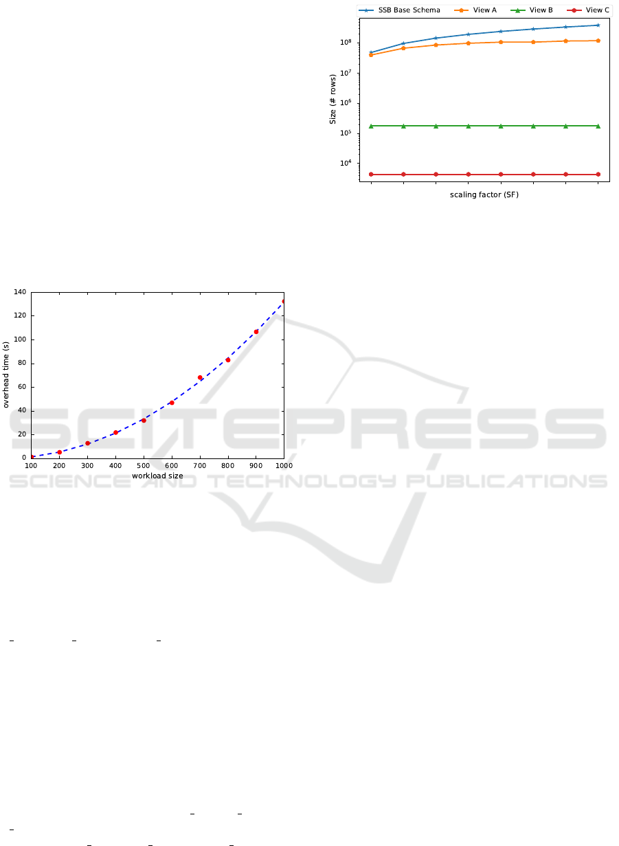
On the other hand, the implementation of the
WPGMA method used in the clustering analysis re-
lies on the nearest-neighbors chain algorithm which
is known to have O(N
2
) time complexity (M
¨
ullner,
2011). As Figure 8 shows, the overhead due to said
analysis features a quadratic growth as the number of
queries in the workload increases, outperforming al-
ternative approaches with exponential complexity dis-
cussed back in section 2.
Figure 8: View selection overhead vs Workload size. The
syntactical analysis features a quadratic growth w.r.t. the
size of the query set.
When it comes to storage cost, view size varies
depending on the cardinality of the fields used in the
group-by clause of their definition (Aouiche et al.,
2006), and whether or not there are hierarchical re-
lations between such attributes (e.g. the one between
c region, c nation and c city). Figure 9 shows
the size per materialized view, as well as the number
of rows in the SSB base schema for a range of values
of the scaling factor (SF). Notice that while the num-
ber of records of views A and C is fairly negligible
in comparison with the base schema, view B and the
base dataset have comparable sizes for small values of
SF. Then, the size of view B tends to stabilize around
10
8
records as the base data set gets larger. Such dif-
ference in size among the views has to do with the car-
dinality of the fields used when defining said views.
For instance, view B uses fields c
city, s city and
d yearmonthnum whose cardinality is far larger than
fields such as c region, c nation and d year, used
in the remaining views.
Figure 9: View size overhead vs SSB scaling factor.
5.4.2 View Selection Performance
With the selected views already materialized, a 100-
query workload was run against each one of the eight
base SSB datasets to get a query latency baseline. Out
of those 100 queries, 75 were covered by the three
available materialized views (25 queries per view),
and the remaining ones were canonical SSB-based
queries. Once the latency baseline was built, the same
workload was issued this time with the query transla-
tion module in place, so that incoming queries match-
ing any of the definitions of the available material-
ized views get rewritten and issued against them. Fig-
ure 10 illustrates the contrast between the baseline
query runtime and the response time when queries run
against materialized views. In the light of these results
it is worth to highlight three key facts:
(i) For all the selected views the time required for
queries to run against the base dataset steadily
grows as the scaling factor (SF) increases from 8
(48 million rows) to 40 (240 million rows). This
describes an expected behaviour since the base
dataset is also growing at a uniform rate (48 mil-
lion rows per step).
(ii) From SF = 48 (288 million rows) onwards, there
is a strong though less regular increase in the av-
erage response time of queries issued against the
base datasets: queries run 5-9 times slower com-
pared to those running on the immediate smaller
dataset (SF = 40), when only a 22-27% mean in-
crease in the query runtime was expected. Such a
stark difference is consequence of Apache Spark
changing the mechanism it uses to implement join
operations. Up to SF = 40, the size of the dimen-
sion tables is small enough for Spark to broad-
cast them across the executors —collocated with
the Hadoop DataNodes— and use its most per-
formant join strategy known as Broadcast Hash
Join. However, for SF ≥ 48 some of those dimen-
Automatic View Selection for Distributed Dimensional Data
25
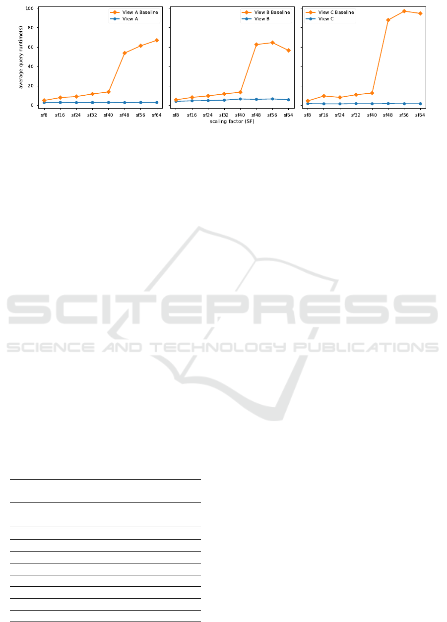
Figure 10: Query runtime per view: Baseline runtime vs. View runtime (|Q | = 100, Spark running on yarn-client mode with
3 executors and spark.executor.memory = 1Gb).
sions grows larger than the threshold set in Spark
for them to be regarded as broadcastable datasets,
compelling Spark to fall back to Sort-Merge Join,
which entails an expensive sorting step on the ta-
bles involved in the join operation, ultimately im-
pacting the query response time.
(iii) Materialized views outperform the base datasets
for any value of SF ≥ 8. Queries running on views
A and C perform 2-8 times faster than the corre-
sponding base dataset for values of SF between 8
and 40, and 22-65 times faster for larger values of
SF. Likewise, queries running against the second
view (view B) run up to 2 times faster than queries
running on the base dataset for SF ≤ 40, and up to
10 times faster for larger values of SF. The expen-
sive join operations performed for queries running
on the base dataset are bypassed for those match-
ing any of the available selected views, allowing
Spark to run those queries in a fraction of their
original query response time.
Table 2 summarizes the results obtained from running
the above test, stating the reduction in query runtime
achieved through each one of the views relative to the
average baseline query runtime.
Table 2: Query latency reduction per view (|Q | = 100).
% Reduction in
query response time
SSB Dataset
size (SF)
View A View B View C
8 40.86 26.99 61.21
16 62.66 42.64 83.36
24 69.05 50.14 80.95
32 75.16 54.48 84.06
40 78.60 51.56 87.05
48 96.02 88.96 98.00
56 96.10 89.15 98.24
64 95.36 89.82 98.46
6 DISCUSSION AND
CONCLUSIONS
The analytical workloads typical in OLAP applica-
tions feature expensive data processing operations
whose cost and complexity increases when running
on a distributed setting. By identifying recurrent op-
erations in the queries composing said workloads and
saving their resulting output on disk or memory in the
form of distributed views, it is possible to speed up the
processing time of not only known but also previously
unseen queries. That is precisely the premise behind
the mechanism detailed in this paper, which leverages
on syntactic analysis of OLAP workloads for iden-
tifying groups of related queries and deriving a lim-
ited but comprehensive set of views out of them. The
views the devised mechanism comes up with proved
an effective method for circumventing expensive dis-
tributed join operations and subsequently reducing the
query processing time by up to 89%–98% with ref-
erence to the runtime on the base distributed dimen-
sional data.
While the convenience of distributed materialized
views is more prominently perceived as the dimen-
sional data grows larger, one of the main open chal-
lenges of the proposed approach has to do with the
unbounded size of the views that the mechanism is
able to compose, which increases the associated pro-
cessing overhead and cuts down the relative benefit of
using these redundant data structures. To cope with
this limitation, the view selection mechanism needs
to be aware not only of the recurrent attributes and
operations of queries but also of the cardinality of
such attributes, so that views including attributes with
high cardinality (consider for instance view B in sec-
tion 5.1) get materialized as multiple size-bounded
child views corresponding to partitions of the origi-
nal view. Additionally, by keeping track of how the
selection conditions of incoming workloads change
IoTBDS 2019 - 4th International Conference on Internet of Things, Big Data and Security
26

over time, it is possible to implement a continuous
view maintenance strategy that performs horizontal
partitioning on the derived views, allowing the pro-
posed mechanism to adapt to workload-specific de-
mands, using an approach similar to the one presented
in (Ordonez-Ante et al., 2017). The implementation
of the cardinality-awareness feature for the proposed
view selection mechanism, as well as the view main-
tenance strategy discussed above are the future exten-
sions of the work presented in this paper.
ACKNOWLEDGEMENTS
This work was supported by the Research Founda-
tion Flanders (FWO) under Grant number G059615N
- “Service oriented management of a virtualised fu-
ture internet” and the strategic basic research (SBO)
project DeCoMAdS under Grant number 140055.
REFERENCES
Aouiche, K. and Darmont, J. (2009). Data mining-based
materialized view and index selection in data ware-
houses. Journal of Intelligent Information Systems,
33(1):65–93.
Aouiche, K., Jouve, P.-E., and Darmont, J. (2006).
Clustering-based materialized view selection in data
warehouses. In Manolopoulos, Y., Pokorn
´
y, J., and
Sellis, T. K., editors, Advances in Databases and In-
formation Systems, pages 81–95, Berlin, Heidelberg.
Springer Berlin Heidelberg.
Camacho Rodriguez, J. (2018). Materialized views in
apache hive 3.0. https://cwiki.apache.org/confluen
ce/display/Hive/Materialized+views. Last accessed:
2018.10.15.
Chirkova, R., Halevy, A. Y., and Suciu, D. (2001). A formal
perspective on the view selection problem. In VLDB
2001, volume 1, pages 59–68.
Derakhshan, R., Stantic, B., Korn, O., and Dehne, F. (2008).
Parallel simulated annealing for materialized view se-
lection in data warehousing environments. In ICA3PP
2008, pages 121–132. Springer.
Friedman, J., Hastie, T., and Tibshirani, R. (2009). Clus-
tering analysis. In The elements of statistical learn-
ing: Data mining, inference and prediction, chap-
ter 14, pages 501–520. Springer series in statistics,
New York.
Gosain, A. and Sachdeva, K. (2017). A systematic review
on materialized view selection. In Satapathy, S. C.,
Bhateja, V., Udgata, S. K., and Pattnaik, P. K., editors,
FICTA 2017, pages 663–671, Singapore. Springer
Singapore.
Goswami, R., Bhattacharyya, D., and Dutta, M. (2017).
Materialized view selection using evolutionary algo-
rithm for speeding up big data query processing. Jour-
nal of Intelligent Information Systems, 49(3):407–
433.
Goswami, R., Bhattacharyya, D. K., Dutta, M., and Kalita,
J. K. (2016). Approaches and issues in view selec-
tion for materialising in data warehouse. International
Journal of Business Information Systems, 21(1):17–
47.
Kumar, T. V. V., Singh, A., and Dubey, G. (2012). Min-
ing queries for constructing materialized views in a
data warehouse. In Advances in Computer Science,
Engineering & Applications, pages 149–159, Berlin,
Heidelberg. Springer Berlin Heidelberg.
M
¨
ullner, D. (2011). Modern hierarchical, agglomerative
clustering algorithms. Computing Research Reposi-
tory (CoRR), abs/1109.2378.
Nalini, T., Kumaravel, A., and Rangarajan, K. (2012).
A comparative study analysis of materialized view
for selection cost. World Applied Sciences Journal
(WASJ), 20(4):496–501.
O’Neil, P. E., O’Neil, E. J., and Chen, X. (2009). The
star schema benchmark (revision 3, june 5, 2009).
https://www.cs.umb.edu/ poneil/StarSchemaB.PDF.
Ordonez-Ante, L., Vanhove, T., Van Seghbroeck, G.,
Wauters, T., Volckaert, B., and De Turck, F. (2017).
Dynamic data transformation for low latency querying
in big data systems. In 2017 IEEE International Con-
ference on Big Data (Big Data), pages 2480–2489.
Phuboon-ob, J. and Auepanwiriyakul, R. (2007). Two-
phase optimization for selecting materialized views in
a data warehouse. International Journal of Computer,
Electrical, Automation, Control and Information En-
gineering, 1(1):119–123.
Plattner, H. (2013). A Course in In-Memory Data Manage-
ment: The Inner Mechanics of In-Memory Databases.
Springer Publishing Company, Inc.
Qushem, U. B., Zeki, A. M., Abubakar, A., and Akleylek,
S. (2017). The trend of business intelligence adoption
and maturity. In UBMK 2017, pages 532–537.
Rousseeuw, P. J. (1987). Silhouettes: a graphical aid to
the interpretation and validation of cluster analysis.
Journal of computational and applied mathematics,
20(1):53–65.
Serna-Encinas, M. T. and Hoyo-Montano, J. A. (2007). Al-
gorithm for selection of materialized views: based on
a costs model. In Current Trends in Computer Sci-
ence, 2007. ENC 2007. Eighth Mexican International
Conference on, pages 18–24. IEEE.
Shvachko, K., Kuang, H., Radia, S., and Chansler, R.
(2010). The hadoop distributed file system. In MSST
2010, pages 1–10, Washington, DC, USA. IEEE Com-
puter Society.
Sun, X. and Wang, Z. (2009). An efficient materialized
views selection algorithm based on pso. In ISA 2009,
pages 1–4. IEEE.
Thakur, G. and Gosain, A. (2011). A comprehensive analy-
sis of materialized views in a data warehouse environ-
ment. International Journal of Advanced Computer
Science and Applications, 2(5):76–82.
Vohra, D. (2016a). Apache avro. In Practical Hadoop
Ecosystem, pages 303–323. Springer.
Automatic View Selection for Distributed Dimensional Data
27

Vohra, D. (2016b). Apache hive. In Practical Hadoop
Ecosystem, pages 209–231. Springer.
Vohra, D. (2016c). Apache parquet. In Practical Hadoop
Ecosystem, pages 325–335. Springer.
Zhang, Q., Sun, X., and Wang, Z. (2009). An efficient
ma-based materialized views selection algorithm. In
CASE 2009, pages 315–318. IEEE.
IoTBDS 2019 - 4th International Conference on Internet of Things, Big Data and Security
28
