Rain Nowcasting from Multiscale Radar Images
Aniss Zebiri
1
, Dominique B
´
er
´
eziat
1
, Etienne Huot
2
and Isabelle Herlin
3
1
Sorbonne Universit
´
e, CNRS, Laboratoire d’Informatique de Paris 6, France
2
Universit
´
e de Versailles Saint-Quentin-en-Yvelines, LATMOS/IPSL, France
3
Inria, France
Keywords:
Rain Forecasting, Weather Radar, Multiscale Image, Image Assimilation, Motion Estimation.
Abstract:
Rainfall forecasting is a major issue for anticipating severe meteorological events and for agriculture manage-
ment. Weather radar imaging has been identified in the literature as the best way to measure rainfall on a large
domain, with a fine spatial and temporal resolution. This paper describes two methods allowing to improve
rain nowcast from radar images at two different scales. These methods are further compared to an operational
chain relying on only one type of radar observation. The comparison is led with regional and local criteria.
For both, significant improvements are quantified compared to the original method.
1 INTRODUCTION
In meteorology, precipitation forecast is a major is-
sue. In case of short term forecast, with a time hori-
zon lower than 2 hours, it is usually called nowcast.
Rainfall nowcast is known to be of major interest for
severe events anticipation (Joe et al., 2012) and for
agriculture (Stigter et al., 2000).
Different rainfall forecasting methods are avai-
lable, ranging from sophisticated numerical weather
prediction (NWP) models to simple extrapolation of
images acquired by satellites or radars. The con-
straints of temporal horizon and spatial scale of the
weather structure dictate the type of methods that can
be successfully applied. NWP models are daily com-
puting weather forecasts: starting from initial condi-
tions that are derived, the future state of the atmosp-
here is estimated from the integration in time of evo-
lution equations. Nowadays, most of NWP models in-
volve data assimilation methods for improving results
from observations (Le Dimet and Talagrand, 1986;
Courtier et al., 1994). The computing time requi-
red by NWPs is usually large and a few hours is re-
quired since the last observations acquisition for pro-
viding a forecast. Assimilating high-resolution data
with a high-resolution NWP model in a short-cycle
mode is a challenging issue that has not yet been re-
ached. On another hand, extrapolation methods ba-
sed on image acquisitions quickly provide an effi-
cient result if the forecast horizon is short enough.
Two types of image extrapolation approaches can be
used, depending on their motion estimation compo-
nent, which is based either on structure tracking or
on dense motion estimation. The tracking appro-
ach (Dixon and Wiener, 1993; Johnson et al., 1998)
first identifies rain structures as characteristic features
of the image and evaluates their displacement by iden-
tifying the same features in successive images, often
with a cross-correlation technique. The dense appro-
ach is based on the optical flow technique (Horn and
Schunk, 1981; B
´
er
´
eziat et al., 2000; Germann and Za-
wadzki, 2002; Bowler et al., 2004; H
´
eas et al., 2007;
Berenguer et al., 2011). However, most motion es-
timation processes do not include a physical model
on the rain evolution and the quality of their results
remain low. During the last decade, an alternative ap-
proach of motion estimation came from the data assi-
milation technique. In the context of rain nowcast,
this image assimilation approach (Le Dimet et al.,
2006; Korotaev et al., 2008; Corpetti et al., 2009; Ti-
taud et al., 2010; Huot et al., 2013) offers the possi-
bility to compute an optimal solution from all types
of information: outputs of an NWP model, satellite
images, radar images, rain gauges measures. Moreo-
ver, motion estimation with image assimilation allows
to combine the dense and feature-based approaches
and relies simultaneously on raw observational ima-
ges and characteristic features, resulting in a better
estimation (Lepoittevin et al., 2013).
In this paper, we describe two methods of multis-
cale rain nowcasting, relying on image assimilation
of images with different spatial resolution. The two
892
Zebiri, A., Béréziat, D., Huot, E. and Herlin, I.
Rain Nowcasting from Multiscale Radar Images.
DOI: 10.5220/0007566908920900
In Proceedings of the 14th International Joint Conference on Computer Vision, Imaging and Computer Graphics Theory and Applications (VISIGRAPP 2019), pages 892-900
ISBN: 978-989-758-354-4
Copyright
c
 2019 by SCITEPRESS – Science and Technology Publications, Lda. All rights reserved

methods derive from an initial work of (Lepoittevin
and Herlin, 2015) that is operationally used by the
French StartUp Weather Measures
1
and referenced as
the RainNowcast (RN) chain in the following. In this
approach, motion is first estimated on a short temporal
window of image acquisitions; then, the last available
image is transported by the velocity map providing a
synthetic image at a chosen time horizon. The first
multiscale method is a serial one: motion estimation
is first estimated from regional images, at small re-
solution, and then refined with local images, at large
resolution. The second method allows to assimilate
simultaneously local and regional images at both re-
solutions.
The paper is organized as follow: Section 2 des-
cribed data and their major characteristics. Section 3
summaries the initial RN method, while Section 4
describes our methodological contributions for com-
bine local and regional data. Section 5 displays results
and evaluates the performance of the multiscale met-
hods both compared to RN results and to the ground
truth. Concluding remarks and future research directi-
ons are given in Section 6.
2 DATA
The radar reflectivity is directly linked to the rain
rate (Marshall and Palmer, 1948). Most of the meteo-
rological radar networks, as the French PANTHERE
network operated by M
´
et
´
eo France include sensors,
providing long distance measures. These radars, usu-
ally working in C or S-BAND frequency ranges, al-
low a large regional coverage. However, their low
spatial resolution (1 km) is a major drawback for local
applications. X-BAND sensors, as operated by Weat-
her Measures, are smaller and provide more accurate
measures but at a shorter range.
The objective is to combine the PANTHERE regi-
onal images with the X-BAND local images for an
improved rain forecast. Both types of images are
acquired each 5 minutes and projected on the same
Cartesian grid at the X-BAND resolution (200 m). Fi-
gure 1 compares PANTHERE to X-BAND images
(the legend gives the color code used to express the
rain rate in mm/h): X-BAND images are more pre-
cise but the PANTHERE domain is larger.
In this paper, we focus on a severe rainfall event
that occurred in June 2016. The set of images has
been acquired between 24
th
at 4 pm and 25
th
at 3 am.
The size of the PANTHER data is 196 × 234 pixels
cropped from the original image and centered over the
1
https://www.weather-measures.fr/
10 20 30 40 50 60 70 80 90 100
20
40
60
80
100
120
140
160
180
200
0
20
40
60
80
100
120
140
160
180
200
0 20 40 60 80 100 120 140 160 180 200
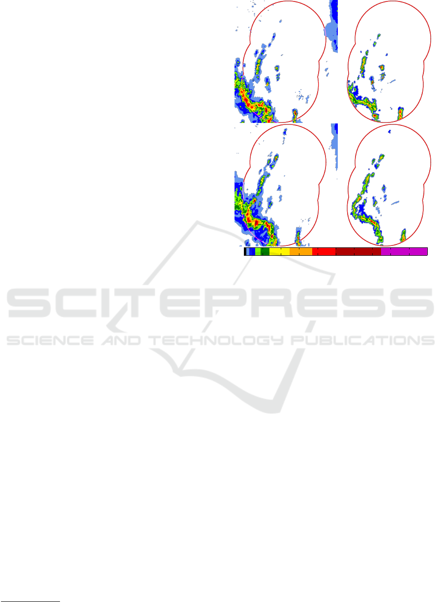
Figure 1: Rainfall event at two spatial resolutions. Left:
PANTHERE data, right: X-BAND data. The red contour
corresponds to the limit of the X-BAND domain. Top:
acquisition at 4 pm. Bottom: at 4:15 pm.
local domain that has a size of 980×1170 pixels. The
local domain covers 64% of the regional domain.
3 RAIN NOWCAST (RN)
This reference method is based on two main steps.
In a first one, a velocity field is estimated from
four consecutive reflectivity radar images. The met-
hod is based on data assimilation and take into ac-
count a model of the dynamics observed by the ima-
ges. It has been proved to be competitive compared
to the classic optical flow based approaches (B
´
er
´
eziat,
2018). Once the velocity map computed, the next step
transports the last image observation, according to the
advection equation, up to the chosen temporal hori-
zon. At each new acquisition, the velocity is updated
and a new forecast is delivered, thanks to a sliding
window technique. The Weather Measures company
runs this process operationally.
In the following subsections, we briefly summa-
rize the method, see (Lepoittevin and Herlin, 2015)
for additional details.
Rain Nowcasting from Multiscale Radar Images
893

3.1 Motion Estimation (ME)
Let define X =

w
T
I

the state vector. w =

u v

T
is the velocity map, I is a synthetic image ha-
ving the same properties than image acquisitions and
T is the transpose operator. (x,t) 7→ X(x,t) is an in-
tegrable function defined over Ω, the image domain,
and on [t
0
,t
3
], the temporal interval of image acquisi-
tion. Observations are reflectivity images. They are
sparse in time. Four observations, denoted O(t
i
) with
i = 0, 1, 2, 3, are used for estimating velocity. Motion
estimation is modeled as the solution of the following
system of equations:
∂X
∂t
(x,t) + (X)(x,t) = 0, (x,t) ∈ Ω×]t
0
,t
3
] (1)
X(x,t
0
) − X
b
(x) = ε
B
(x) (2)
(X)(x,t) − O(x,t) = ε
R
(x,t), if t = t
i
. (3)
The first equation, Eq. (1), describes the temporal dy-
namics of the state vector and the knowledge available
on studied the system, either physical laws or heuris-
tics hypothesis. Here, we assume:
1. the synthetic image I is transported by the velo-
city map w. This is modeled by the advection
equation:
∂I
∂t
(x,t) + ∇I(x,t).w(x,t) = 0 with ∇
the gradient operator,
2. the velocity is stationary on a short time interval,
so:
∂w
∂t
(x,t) =
~
0;
With such hypothesis, is defined by (X) =

~
0 ∇I.w

T
.
The second equation, Eq. (2), describes the know-
ledge given on the initial condition of the state vector,
X(t
0
). X
b
is called background. I
b
is taken as the first
available image observation, I
b
(t
0
) = O(t
0
), and w
b
is
either
~
0 or the value estimated on the previous win-
dow in the sliding window process. ε
B
is supposed
unbiased Gaussian and its covariance matrix B is cho-
sen as follow:

∞ 0
0 B
I

. In others words, w(t
0
) is
not constrained to remain close to w
b
.
In Eq. (3), stands for the observation operator:
it projects the state vector in the vectorial space of the
observations. In this particular case, (X) = I. The
equation Eq. (3) expresses that the synthetic images I
should be close to the images acquired at times t
i
. ε
R
is also supposed unbiased Gaussian and described by
its covariance matrix R.
Eqs. (1,2,3) are solved with a variational approach
by minimizing the cost function J:
J(X(t
0
)) =
Z
Ω
ε
B
(x)
T
B(x)
−1
ε
B
(x)dx+
Z
Ω
Z
t
3
t
0
ε
R
(x,t)
T
R
−1
(x,t)ε
R
(x,t)dxdt
(4)
with the constraint of Eq. (1). It has been
shown (Le Dimet and Talagrand, 1986) that gradient
of J is:
∇J = B
−1
(X(t
0
) − X
b
) + λ(t
0
) (5)
where λ is the adjoint variable, defined by:
λ(x,t
3
) = 0 (6)
−
∂λ
∂t
(x,t) +

∂
∂X

∗
λ(x,t) =

∂
∂X

∗
R
−1
(x,t)
× ( (X)(x,t) − O(x,t))
(7)

∂
∂X

∗
is the adjoint operator. It is formally defined
as the dual operator of
∂
∂X
and the same applies for

∂
∂X

∗
. Reader should notice that the computation
of λ(x,t) is backward in time, from t
3
up to t
0
. The
approach is named 4D-Var (Courtier et al., 1994) in
the data assimilation literature.
ME obtained with a variational data assimilation
technique is summarized in Algorithm 1.
Algorithm 1: Motion Estimation (ME).
Require: : X
b
,O(t
1
),O(t
2
),O(t
3
),B, R, MaxIter
1: Set the iteration index k = 0
2: Initial condition of state vector X
k
(t
0
) = X
b
3: repeat
4: Forward integration: compute X
k
(t) for all
time with Eq. (1), and compute J
k
5: Backward integration: compute λ
k
(t) for all
time with Eqs. (6,7) and compute ∇J
k
6: Update state vector X(t
0
) with the L-BFGS
solver:
X(t
0
)
k+1
= LBFGS(X(t
0
)
k
,J
k
,∇J
k
)
7: k=k+1
8: until |∇J
k
| < ε or k > MaxIter
9: return X(t
0
)
k
The numerical implementation of the model is
obtained with finite difference techniques and a semi-
Lagrangian scheme. The discrete adjoint of the dis-
crete model is obtained from an automatic diffe-
rential software. The choice of the covariance matri-
ces values B and R depends on the type of data and is
discussed in Section 5.
VISAPP 2019 - 14th International Conference on Computer Vision Theory and Applications
894

3.2 Forecasting
The last available observation O(t
3
) is then extrapo-
lated over time, thanks to the velocity map computed
by the ME algorithm, w
ME
: Eq. (1) is integrated in
time from its initial condition:
X(t
3
) =

w
ME
O(t
3
)

(8)
∂X
∂t
(x,t) +
f
(X)(x,t) = 0 ∀t > t
3
(9)
If the time horizon is large, the hypothesis of statio-
nary motion is no more valid and the heuristic of La-
grangian constancy of w is chosen. This is described
by the non-linear advection equation
∂w
∂t
+∇w.w = 0.
The numerical model is then slightly modified to
obtain
f
=

∇w.w ∇I.w

T
with non-linear ad-
vection on w, see (Lepoittevin and Herlin, 2015).
4 MULTISCALE RAIN
NOWCASTING
4.1 Sequential Approach for ME
This section presents a first approach for the estima-
tion of motion from multiscale image, with the ob-
jective of improving the performance of Rain Now-
cast, thanks to the simultaneous use of local and regi-
onal data. In the following we both make use of re-
gional data, denoted by a r exponent, and local data,
denoted by a l exponent. Motion estimation inclu-
des two phases. In the first phase, the motion field
w
r
is estimated from the regional images. w
r
is then
oversampled to the local resolution, and used as back-
ground for the second phase: motion estimation on
the local image. This second phase computes a refi-
nement of the regional estimation from the local data
with a finer spatial resolution. Algorithm 2 illustra-
tes the principle of the method, where ↑ stands for the
oversampling operator.
This approach is fully sequential as it requires the
estimation of the regional motion field before com-
puting the local one. As pointed out in the previ-
ous section, motion estimation includes a set of pa-
rameters depending on the type of input data. In this
sequential approach, the two phases apply indepen-
dently, consequently allowing to define independent
parameters, suited for the data types.
Algorithm 2: Sequential Multiscale Motion Estimation.
1: Read the regional acquisitions O
r
(t
i
)
i={0,1,2,3}
2: Set the values of regional covariance matrices B
r
and
R
r
3: Set the initial background
X
r
b
= (
w
r
(t
0
) O
r
(t
0
)
)
T
4: Regional estimation
X
r
(0) = ME(X
r
b
,O
r
(t
i
)
i={1,2,3}
,B
r
,R
r
,MaxIter)
5: Oversample the regional estimation to local resolu-
tion (1 km to 200 m) w
l
(t
0
) =↑ w
r
(t
0
)
6: Read the local acquisitions O
l
(t
i
)
i={0,1,2,3}
7: Set the values of local covariance matrices B
l
, R
l
8: Set the initial background
X
l
b
=

w
l
(t
0
) O
l
(t
0
)

T
9: Local refinement
X(0) = ME(X
l
b
,O
l
(t
i
)
i={1,2,3}
,B
l
,R
l
,MaxIter)
4.2 Parallel Approach for ME
Another way to tackle this problem is to simultane-
ously assimilate local and regional data: the image
acquisitions of the two radars do not have the same
spatial resolution but they are assimilated for produ-
cing a velocity map at the X-BAND resolution. The
regional data of PANTHER are then first oversampled
at the local resolution. A Gaussian blur, with a stan-
dard deviation of 5, is then applied on the result for
avoiding the aperture problem (Beauchemin and Bar-
ron, 1995) occurs when pixels are duplicated with the
same value. At that stage, local and regional data have
the same resolution and can be simultaneously assimi-
lated with the model.
The state vector is extended with a fourth compo-
nent I
r
: a synthetic image having the same resolution
than the local data and close to values of the regional
data. The synthetic local data is denoted I
l
. The state
vector is given by:
X(x,t) =


w(x,t)
I
l
(x,t)
I
r
(x,t)


(10)
With the same formalism and notations than Sub-
section 3.1, we extend the operators and . The
evolution of the state vector is given by:
∂w
∂t
+ ∇w.w = 0 (11)
∂I
l
∂t
+ ∇I
l
.w = 0 (12)
∂I
r
∂t
+ ∇I
r
.w = 0 (13)
Rain Nowcasting from Multiscale Radar Images
895

and (X) =

~
0 ∇I
l
.w ∇I
r
.w

T
. (X) writes:
(X) =

I
l
I
r

T
(14)
Observations are given by a 2-component image
including the local and regional data: O(t) =

O
l
(t) O
r
(t)

T
. The covariance matrix R is then de-
fined by:
R =

R
l
0
0 R
r

(15)
The background value X
b
is exten-
ded to

w
b
I
l
b
I
r
b

T
and initialized by:

w
b
O
l
(t
0
) O
r
(t
0
)

. The covariance matrix
B writes:


∞ 0 0
0 B
I
r
0
0 0 B
I
l


. (16)
The challenge of this approach is to accurately
tune the covariance matrices between the local and the
regional scales. This method has the advantage to be
faster than the sequential one, especially if distributed
on several cores.
4.3 Multiscale Forecasting
The process of forecasting in a multiscale context is
similar to the one described in Subsection 3.2. Both
local and regional data are extrapolated in time using
the velocity map computed by one of the two multis-
cale methods. Computing the forecast both local and
regional scale allows to evaluate the methods from
different criteria, as discussed in the next section.
5 RESULTS
For evaluating the two multiscale methods, deno-
ted SMRN for Sequential Multiscale Rain Nowcas-
ting and PMRN for Parallel Multiscale Rain Now-
casting, we compare their forecast results with those
of Rain Nowcasting (RN), described in Section 3.
The following four metrics are taken from the state-
of-the-art (Shi et al., 2017): probability of detection
(POD), Figure Merit in Space (FMS), False Alarm
Rate (FAR) and Mean Absolute Error (MAE).
Pixels from the forecasted and ground truth ima-
ges are classified as rain (1) and no-rain (0). The
number of true positive T P (prediction=1, ground
truth=1), true negative T N (prediction=0, ground
truth=0), false positive FP (prediction=1, ground
truth=0) and false negative FN (prediction=0, ground
truth=1) is then calculated. Three metrics derive from
theses values: POD =
T P
T P+F N
that measures the over-
lapping between observed structures and correct fo-
recasted structures, FMS =
T P
FP+F N+T P
that measures
the overlapping between observed structures and fo-
recasted structures, and FAR =
FP
FP+T N
that measures
the overlapping between wrong forecasted structures
and forecasted structures. The last metric, MAE, is
defined as the average squared error between the pre-
dicted rain rate and the observed one (ground truth).
If good quality results, POD and FMS should be high,
FAR and MAE low.
As two scales of images are included in the pro-
cess, there are two ways for evaluating the methods.
The first one compares the output of SMRN or PRMN
with the output of RN obtained on local data. This al-
lows to quantify the benefit of regional data. The me-
trics are then computed on the forecasted local data
and on the local domain (the circular domains of the
three X-BAND radars as showed in Figure 1). This is
discussed in Subsection 5.1. The second way compa-
res the output of SMRN or PRMN with the output of
RN computed on regional data. This allows to quan-
tify enhancement of regional data by local data. In
that case, the metrics are computed on the forecasted
regional data but still on the local domain. This is
discussed in Subsection 5.2.
Our data set is divided in three sequences with
a total of 612 images for both scales. In this pa-
per the statistics and figures only come from the se-
cond event (24 to 25th June, 2016). Nevertheless the
results for the two other sequences remains similar.
This sequence is chosen for two reasons: first, obser-
ved events are quite typical; second, several cells are
visible with high velocities.
5.1 Evaluation on Local Spatial Domain
An important requirement of the method is the tuning
of the parameters. In particular, matrices B
l
I
, B
r
I
, R
l
and R
r
should be correctly initialized according to the
type of data. In this application, the tuning concerns
the precision on the rain values. R
l
(x,t
i
) is conse-
quently taking into account the rain/no-rain classifica-
tion: high value if no-rain, low value otherwise. This
means that only significant rainfall quantities will be
assimilated. The same applies for R
r
and regional
data. B
l
I
and B
r
I
are set to a low value. This means
that the I component of the state vector is forced to be
close to local and regional backgrounds.
We display on Figures 2 and 3 the four chosen me-
trics for the results of SMRN and PMRN compared
to RN, when computing a forecast at 15 minutes hori-
zon from each image of the sequence (apart the first 6
ones that are used for initializing the sliding window:
VISAPP 2019 - 14th International Conference on Computer Vision Theory and Applications
896

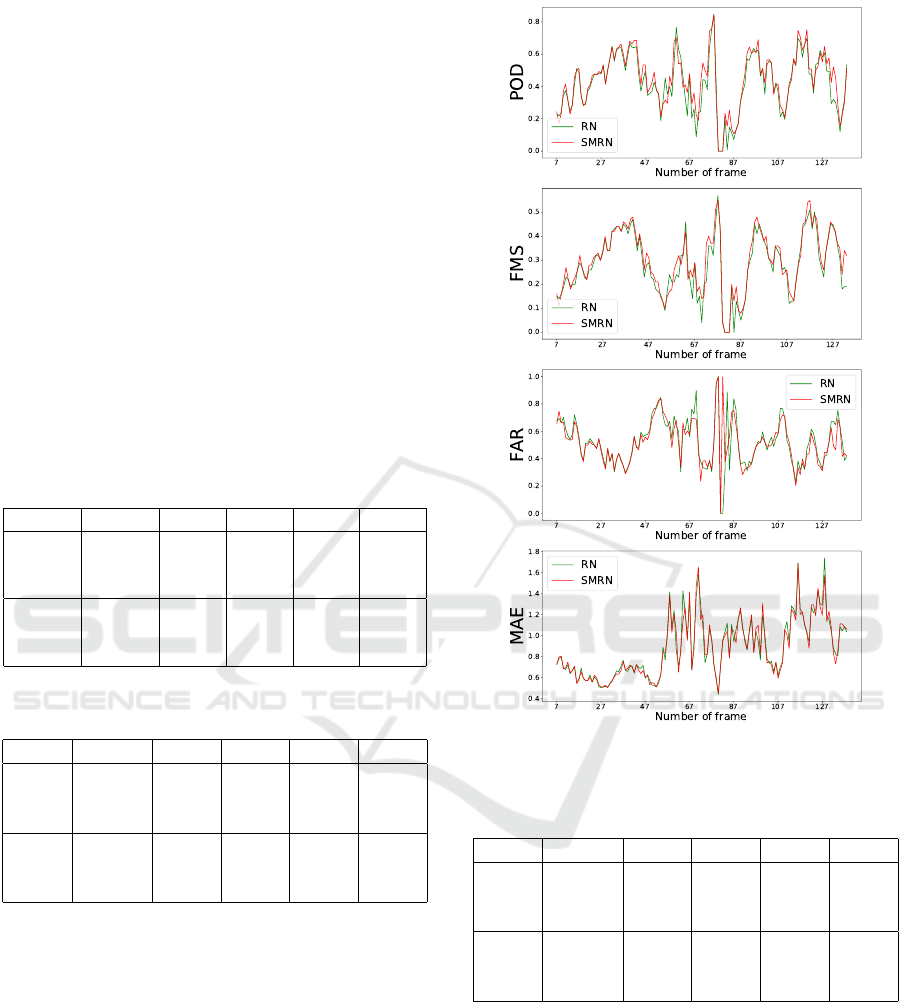
graphics begin at 7). We also computed the forecasts
at 1 hour and 15 minutes horizon (making the com-
parison with ground truth not possible on the last 10
ones: graphics end at 138).
The part on local data of Table 1 gives the statis-
tics for the whole sequence and shows that the perfor-
mances of SMRN and PMRN are better than those of
RN. This is first due to the fact that the motion of the
structures located on the boundary of the local dom-
ain (purple contours depicted in Figure 4) is better es-
timated if making use of the regional data. Moreover,
the quantity of forecasted rain is more accurate if it
is entering the local domain: it is estimated from the
rain that is observed on regional data outside the lo-
cal domain. Statistics given in Table 2 confirm this
improvement. Another improvement is a better esti-
mation of motion inside the local domain, leading to
a better forecast: forecasted rain structures are more
correlated to the ground truth.
Table 1: Comparison of average scores on local and regio-
nal data.
POD FMS FAR MAE
Local
data
RN 0.421 0.270 0.522 0.885
SMRN 0.445 0.290 0.513 0.880
PMRN 0.438 0.290 0.511 0.877
Reg.
data
RN 0.439 0.332 0.423 0.682
SMRN 0.475 0.365 0.386 0.665
PMRN 0.442 0.342 0.390 0.674
Table 2: Comparison of metrics scores with local data on
06/24/2016 at 07:45 and on 06/25/2016 at 17:35.
POD FMS FAR MAE
06/24
07:45
RN 0.608 0.420 0.417 1.740
SMRN 0.648 0.420 0.448 1.573
PMRN 0.654 0.440 0.415 1.707
06/25
17:35
RN 0.346 0.190 0.702 0.695
SMRN 0.373 0.210 0.667 0.684
PMRN 0.348 0.190 0.688 0.663
5.2 Evaluation on Regional Spatial
Domain
The forecast performances are now analyzed in com-
parison with the regional data. The goal is to evaluate
the benefit of adding local data for regional forecas-
ting applications. Local and regional covariance ma-
trices R and B are set to the same values than in the
previous subsection.
It can be seen on Figures 5, 6 and in the regio-
nal part of Table 1 that SMRN and PMRN provide
the best results. Improvements are located inside the
local domain: the forecasted rain structures are better
correlated to the ground truth as illustrated in Figure 7
Figure 2: Results of SMRN at 15 minutes horizon on local
data.
Table 3: Comparison of metrics scores with regional data
on 06/24/2016 at 07:45 and on 06/25/2016 at 17:35.
POD FMS FAR MAE
06/24
07:45
RN 0.623 0.500 0.276 1.294
SMRN 0.668 0.540 0.244 1.182
PMRN 0.649 0.530 0.250 1.291
06/25
17:35
RN 0.271 0.200 0.544 0.604
SMRN 0.356 0.270 0.457 0.554
PMRN 0.315 0.240 0.479 0.617
and Table 3. This is due to the better accuracy of the
local data (better spatial resolution) compared to the
regional ones. Outside the local domain, the regional
data being the only available, the use of local data by
our approach does not impact the results of SMRN
and PMRN.
Rain Nowcasting from Multiscale Radar Images
897

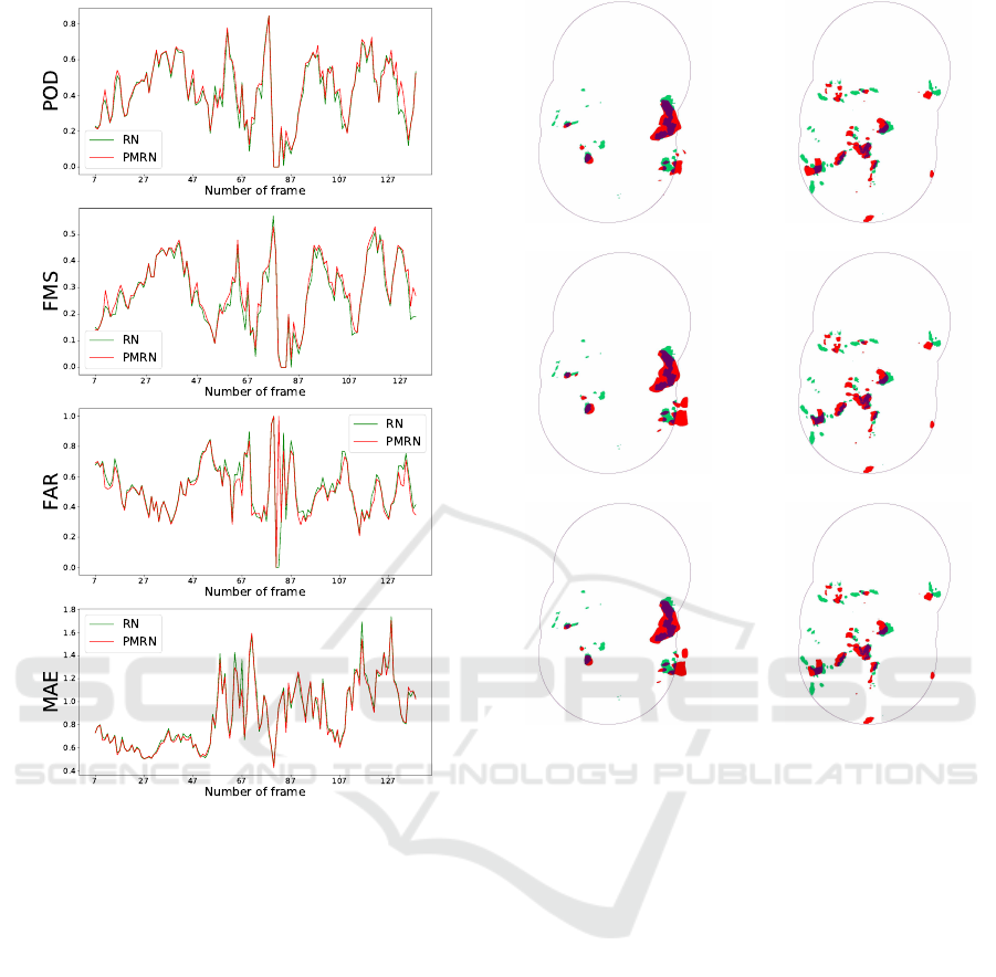
Figure 3: Results of PMRN at 15 minutes horizon on local
data.
6 CONCLUSION AND FUTURE
WORKS
This paper described two rain nowcast multiscale
method applied on two types of radar data: regio-
nal data with a rough spatial resolution and local data
with a fine spatial resolution, on a smaller spatial
domain. We showed the improvement of these multis-
cale methods compared to an operational one applied
on only local high resolution data. We illustrated the
performance of these approaches when forecasting at
a short temporal horizon of 15 minutes. Up to 45 mi-
nutes, conclusions remain quite similar but the quality
of forecast decreases.
Over 45 minutes, our methods provide low quality
results, due to the numerical scheme chosen for ap-
proximating advection of motion and reflectivity data
during the forecast process. This semi-Lagrangian
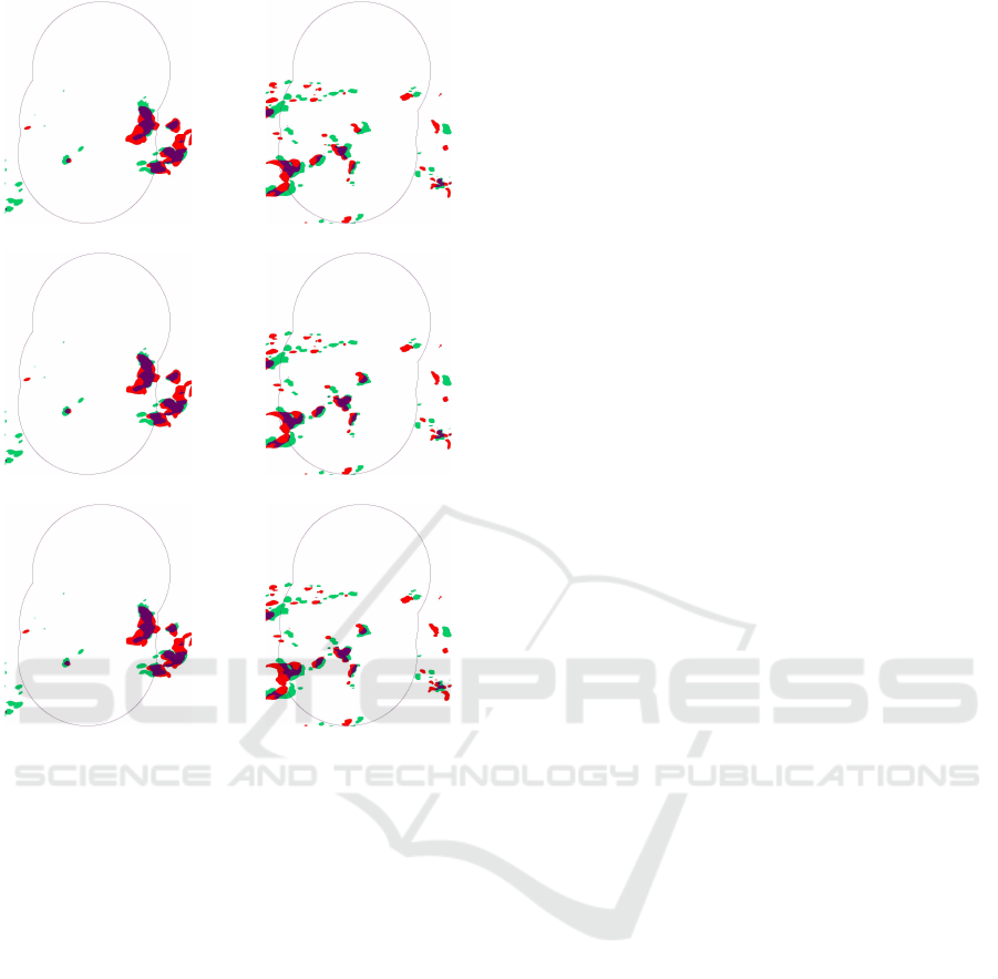
(a) RN
(b) SMRN
(c) PMRN
Figure 4: 15 minutes horizon forecast for local data compu-
ted by RN, SMRN and PMRN. Left column: on 06/24/2016
at 07:45, right column: on 06/25/2016 at 17:35. Ground
truth is in green, forecast in red and their intersection in
purple.
scheme, being implicit, has the major advantage not
be constrained to CFL conditions. This allow using
a high value time step and consequently reducing
the global computational requirements. However,
this scheme has the drawback to smooth (and conse-
quently to suppress) the rain structures if applied for
a long temporal horizon. In a future work, alternative
numerical schemes will be investigated.
Another issue concerns the lower performance of
PMRN compared to SMRN one. However, PMRN
remains promising because it is faster than SMRN.
Additional research work should be considered for the
definition of the covariance matrix R. Radars from
the PANTHERE regional network do not see the same
structures than the local X-BAND radars: the altitude
of the signal acquisition is depending on the distance
between the radar and the rainfall event. This property
may introduce contradictions during the optimization
phase of data assimilation as a unique motion field is
VISAPP 2019 - 14th International Conference on Computer Vision Theory and Applications
898

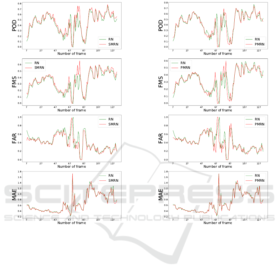
Figure 5: Results of SMRN forecast at 15 minutes horizon
on regional data.
not able to correspond to different structures in the
local and regional data. A weighting coefficient must
be applied between the local and regional data that
should be expressed by the matrices R
l
and R
r
.
ACKNOWLEDGMENTS
This research work is funding by the company Weat-
her Measures.
REFERENCES
Beauchemin, S. and Barron, J. (1995). The computation of
optical flow. ACM Computing Surveys, 27(3).
Berenguer, M., Sempere-Torres, D., and Pegram, G. G.
(2011). Sbmcast – an ensemble nowcasting techni-
que to assess the uncertainty in rainfall forecasts
Figure 6: Results of PMRN forecast at 15 minutes horizon
on regional data.
by lagrangian extrapolation. Journal of Hydrology,
404(3):226 – 240.
B
´
er
´
eziat, D., Herlin, I., and Younes, L. (2000). A Generali-
zed Optical Flow Constraint and its Physical Interpre-
tation. In Proceedings of the conference on Computer
Vision and Pattern Recognition, volume 2, pages 487–
492, Hilton Head, SC, United States. IEEE.
B
´
er
´
eziat, Herlin, I. (2018). Motion and acceleration from
image assimilation with evolution models. Digital
Signal Processing, 83:45–58.
Bowler, N., Pierce, C., and Seed, A. (2004). Development
of a rainfall nowcasting algorithm based on optical
flow techniques. Journal of Hydrology, 288:74–91.
Corpetti, T., H
´
eas, P., Memin, E., and Papadakis, N. (2009).
Pressure image assimilation for atmospheric motion
estimation. Tellus A, 61(1):160–178.
Courtier, P., Th
´
epaut, J.-N., and Hollingsworth, A. (1994).
A strategy for operational implementation of 4D-Var,
using and incremental approach. Quaterly Journal of
the Royal Meteorological Society, 120(1367–1387).
Dixon, M. and Wiener, G. (1993). Titan: Thunderstorm
identification, tracking, analysis, and nowcasting—a
Rain Nowcasting from Multiscale Radar Images
899

(a) RN
(b) SMRN
(c) PMRN
Figure 7: 15 minutes horizon forecast for regional data
computed by RN, SMRN and PMRN. Left column: on
06/25/2016 at 17:35, right column: on 06/24/2016 at 07:45.
radar-based methodology. Journal of Atmospheric
and Oceanic Technology, 10:785.
Germann, U. and Zawadzki, I. (2002). Scale-dependence
of the predictability of precipitation from continen-
tal radar images. part i: Description of the metho-
dology. Monthly Weather Review - MON WEATHER
REV, 130.
H
´
eas, P., Memin, E., Papadakis, N., and Szantai, A. (2007).
Layered estimation of atmospheric mesoscale dyn-
amics from satellite imagery. IEEE Transactions
on Geoscience and Remote Sensing, 45(2)(12):4087–
4104.
Horn, B. and Schunk, B. (1981). Determining optical flow.
Artificial Intelligence, 17:185–203.
Huot, E., Herlin, I., and Papari, G. (2013). Optimal Ort-
hogonal Basis and Image Assimilation: Motion Mo-
deling. In ICCV - International Conference on Com-
puter Vision, Sydney, Australia. IEEE.
Joe, P., Dance, S., Lakshmanan, V., Heizenreder, D., James,
P., Lang, P., Hengstebeck, T., Feng, Y., Li, P., Yeung,
H.-Y., Suzuki, O., Doi, K., and Dai, J. (2012). Au-
tomated processing of doppler radar data for severe
weather warnings. In Bech, J. and Chau, J. L., editors,
Doppler Radar Observations, chapter 2. IntechOpen,
Rijeka.
Johnson, J. T., MacKeen, P. L., Witt, A., Mitchell, E. D. W.,
Stumpf, G. J., Eilts, M. D., and Thomas, K. W. (1998).
The storm cell identification and tracking algorithm:
An enhanced wsr-88d algorithm. Weather and Fore-
casting, 13(2):263–276.
Korotaev, G. K., Huot, E., Le Dimet, F.-X., Herlin, I., Stani-
chny, S., Solovyev, D., and WU, L. (2008). Retrieving
ocean surface current by 4-D variational assimilation
of sea surface temperature images. Remote Sensing
of Environment, 112(4):1464–1475. Remote Sensing
Data Assimilation Special Issue.
Le Dimet, F.-X., Antoniadis, A., Ma, J., Herlin, I., Huot, E.,
and Berroir, J.-P. (2006). Assimilation of images in
geophysical models. In Conference on International
Science and Technology for Space, Kanazawa, Japan.
Le Dimet, F.-X. and Talagrand, O. (1986). Variational al-
gorithms for analysis and assimilation of meteorologi-
cal observations: Theoretical aspects. Tellus, 38A:97–
110.
Lepoittevin, Y., B
´
er
´
eziat, D., Herlin, I., and Mercier, N.
(2013). Continuous tracking of structures from an
image sequence. In VISAPP - 8th International Con-
ference on Computer Vision Theory and Applications,
pages 386–389, Barcelone, Spain. Springer Verlag.
Lepoittevin, Y. and Herlin, I. (2015). Assimilation of ra-
dar reflectivity for rainfall nowcasting. In IGARSS -
IEEE International Geoscience and Remote Sensing
Symposium, pages 933–936, Milan, Italy.
Marshall, S. and Palmer, K. (1948). The distribution of rain-
drops with size. .J. Metrol., 5.
Shi, X., Gao, Z., Lausen, L., Wang, H., and Yeung, D.-Y.
(2017). Deep learning for precipitation nowcasting:
A benchmark and a new model. In 31st Conference
on Neural Information Processing Systems.
Stigter, C. J., Sivakumar, M. V. K., and Rijks, D. A.
(2000). Agrometeorology in the 21st century: works-
hop summary and recommendations on needs and
perspectives. Agricultural and Forest Meteorology,
103(1/2):209–227.
Titaud, O., Vidard, A., Souopgui, I., and Le Dimet, F.-X.
(2010). Assimilation of Image Sequences in Numeri-
cal Models. Tellus A, 62(1):30–47.
VISAPP 2019 - 14th International Conference on Computer Vision Theory and Applications
900