Learning of Activity Cycle Length based on Battery Limitation in

Multi-agent Continuous Cooperative Patrol Problems

Ayumi Sugiyama, Lingying Wu and Toshiharu Sugawara

Department Computer Science and Communications Engineering, Waseda University, Tokyo 1698555, Japan

Keywords:

Continuous Cooperative Patrol Problem, Cycle Learning, Multi-agent, Division of Labor, Battery Limitation.

Abstract:

We propose a learning method that decides the appropriate activity cycle length (ACL) according to environ-

mental characteristics and other agents’ behavior in the (multi-agent) continuous cooperative patrol problem.

With recent advances in computer and sensor technologies, agents, which are intelligent control programs

running on computers and robots, obtain high autonomy so that they can operate in various ﬁelds without

pre-deﬁned knowledge. However, cooperation/coordination between agents is sophisticated and complicated

to implement. We focus on the ACL which is time length from starting patrol to returning to charging base

for cooperative patrol when agents like robots have batteries with limited capacity. Long ACL enable agent

to visit distant location, but it requires long rest. The basic idea of our method is that if agents have long-life

batteries, they can appropriately shorten the ACL by frequently recharging. Appropriate ACL depends on

many elements such as environmental size, the number of agents, and workload in an environment. Therefore,

we propose a method in which agents autonomously learn the appropriate ACL on the basis of the number

of events detected per cycle. We experimentally indicate that our agents are able to learn appropriate ACL

depending on established spatial divisional cooperation.

1 INTRODUCTION

With recent developments in technology, we can ex-

pect that agents, that are autonomous programs con-

trolling robots and computer systems, often have to

collaborate and coordinate with each other to solve

complicated and sophisticated problems. However,

creating methods for establishing cooperation among

multiple agents is challenging due to the difﬁculty

of realizing advanced autonomy and various com-

plex interaction patterns between agents. In partic-

ular, it is crucial to estimate others’ strategies for co-

operation between agents that have their own behav-

ioral strategies and different computational costs. In

tackling these issues, the multi-agent patrol problem

(MAPP) has attracted attention as a good case study

on many multi-agent systems because it has essen-

tial issues such as autonomy, dispersibility, commu-

nication restriction, and scalability, all of which are

required to realize intelligent autonomous distributed

systems (David and Rui, 2011).

We also extend this problem to the continuous

cooperative patrol problem (CCPP) in which multi-

ple autonomous agents with limited battery capacities

continuously move around in an environment where

events occur at a certain probability (Sugiyama and

Sugawara, 2017). In the MAPP, all nodes (locations)

are visited with the same priority/frequency because

the purpose of MAPP is to minimize idleness which

is the interval of two visits for every node. In com-

parison, agents in the CCPP are required to visit in-

dividual nodes with different visitation requirements,

which reﬂect that events in nodes occur with different

probabilities or reﬂect the importance of nodes. Thus,

high visitation requirements indicate, for example, lo-

cations that require a high-security level at which no

events must be missed in security patrolling applica-

tions. Thus, the objective of agents in the CCPP is

to minimize the duration of unawareness which is the

length of time for which agents leave occurred events

unaware without visiting the locations.

Thus, because of the importance of these prob-

lems, a number of studies have tackled MAPPs and

CCPPs in multi-agent system contexts. For example,

Cheva (Chevaleyre, 2005) classiﬁed various classes

of patrolling strategies and compared these strategies.

David and Rui (David and Rui, 2011) summarized

developments of patrolling methods and indicated is-

sues that must extensively be studied regarding the

MAPPs. We (Sugiyama et al., 2016) also proposed

Sugiyama, A., Wu, L. and Sugawara, T.

Learning of Activity Cycle Length based on Battery Limitation in Multi-agent Continuous Cooperative Patrol Problems.

DOI: 10.5220/0007567400620071

In Proceedings of the 11th International Conference on Agents and Artiﬁcial Intelligence (ICAART 2019), pages 62-71

ISBN: 978-989-758-350-6

the learning method, in which agents individually de-

cide where they should work using lightweight com-

munications and using the learning which locations

they should visit more frequently than others. They

found that the agents with their methods could ef-

fectively move around the environment by identify-

ing their responsible areas, i.e., they ﬁnally formed a

certain cooperation structure based on the division of

labors.

Although this method could be used to efﬁciently

patrol an environment to detect events in it, we found

that agents have to coordinate their behavior by taking

into account the interval of visits. Because we assume

that agents are (the control programs of) robots, they

often stop operation for battery charging and/or peri-

odic inspections. This interruption in operation may

negatively affect patrolling, such as security surveil-

lance. Because temporarily stopping for charging is

frequent and inevitable in actual operation, strategic

behavior is required to minimize the inﬂuence of stop-

ping by taking into account robots’ noise and the char-

acteristics of the areas in which they move around.

Although a few studies discussed the battery capac-

ity of agents (robots) (Sipahioglu et al., 2010; Jensen

et al., 2011; Bentz and Panagou, 2016), the appro-

priate timing for when to return to charge and when

to resume operation for autonomous agents was not

clariﬁed in their methods.

A cyclic strategy, in which agents move until the

batteries become empty and then charge to make the

batteries full in different periodic phases, is one of the

simplest ways to minimize the duration of unaware-

ness in the CCPP. In this paper, a sequence of actions

from the agent leaving the charging base with a full

battery, moving around the environment, returning to

the base and completing the charge is called a round

and the time length of the moving in a round is called

activity cycle length (ACL). Performance of a cyclic

strategy depends on a battery capacity. For example,

agents with a small battery capacity cannot cover dis-

tant tasks/events, and the cumulative return cost for

recharging is high in a large environment due to fre-

quent charging. In contrast, agents with long-life bat-

teries can be expected to move more effectively and

cover distant events but they must stop operations for

a long time for recharging, resulting in a long duration

of unawareness. Therefore, because appropriate ACL

may depend on the environmental characteristics and

behaviors of other cooperative agents, agents are re-

quired to autonomously learn which ACL will lead

to better results through actual cooperative behavior

from the viewpoint of the entire performance.

In this paper, we extend the method proposed in

(Sugiyama et al., 2016) to learn appropriate ACL

in the CCPP model in order to adapt other agents’

cooperative strategies (including their ACL) and the

characteristics of the areas in which individual agents

mainly move around. In this method, we assume that

agents have long-life batteries and they can adaptively

decide their ACL by returning/restarting regardless of

their remaining battery capacities, because it is easy

to shorten ACL. Of course, they must not run out of

battery during operations. The features of our method

is that, like the method in (Sugiyama et al., 2016),

it does not require tight communication and deep in-

ference for cooperation, meaning that frequent mes-

sage exchange and the sophisticated reasoning of oth-

ers’ internal intentions are not used; this makes our

method efﬁcient and lightweight, and thereby, our

method is applicable to dynamic environments. We

experimentally indicate that agents with our method

are able to identify appropriate ACL. Furthermore, we

found that agents established a spatial division of la-

bor, as in (Sugiyama et al., 2016); thus, agents in-

dividually identify where they should move around

as the nodes they are responsible for. This enables

agents to decide ACL differently and appropriately

for their own speciﬁc situations.

2 RELATED WORK

Various approaches, especially approaches based on

reinforcement learning for the MAPP and CCPP,

are examined so far. David and Rui (David and

Rui, 2011) summarized the development of patrolling

methods. They stated that non-adaptive solutions

such as methods based on the traveling salesman

problem often outperform other solutions in many

cases except in large or dynamic environments. To

adapt to these environments, they insisted that agents

must have high autonomy. Machado et al. (Machado

et al., 2003) evaluated reactive agents and cognitive

agents that have different depths to analyze patrol

graphs and investigated the characteristics of these

agents. In actual patrol problems, because cogni-

tive agents have greater perception, they can do more

sophisticated operations due to recent developments

in technology. Santana et al. (Santana et al., 2004)

modeled a patrolling task as a reinforcement learn-

ing problem and proposed adaptive strategies for au-

tonomous agents. Then, they showed that their strate-

gies were not always the best but were superior in

most of the experiments.

The CCPP assumes a dynamic environment in

which events occur with certain probabilities and the

duration of unawareness is considered instead of idle-

ness as in the MAPP. Ahmadi and Stone (Ahmadi and

Learning of Activity Cycle Length based on Battery Limitation in Multi-agent Continuous Cooperative Patrol Problems

Stone, 2006), by assuming that events to be found

were generated stochastically, proposed agents that

learn the probability of events and adjust their area of

responsibility to minimize the average required time

to detect events. Chen and Yum (Chen and Yum,

2010) modeled a patrolling environment with a non-

liner security level function in the context of a security

problem. In this model, agents have to visit each node

with a different frequency according to the values

of the function. Pasqualetti et al. (Pasqualetti et al.,

2012) studied a patrol problem in which all nodes

have different priorities, but their model was a simple

cyclic graph with a small number of nodes. Popescu

et al. (Popescu et al., 2016) proposed a patrolling

method for a wireless sensor network in which agents

collect saved data from sensors with limited storage

independently. Agents in this model decide the prior-

ities of nodes to visit on the basis of the accumulated

amount of data and data generation rate.

Sugiyama et al. (Sugiyama et al., 2016) proposed

a method called the adaptive meta-target decision

strategy with learning of dirt accumulation probabili-

ties (AMTDS/LD) by combining the learning of a tar-

get decision strategy in the planning process and the

learning of the importance of each location for clean-

ing tasks. Agents with AMTDS/LD indirectly coop-

erate with other agents by learning the importance of

nodes, which is partly taken into account reﬂects the

visiting frequencies of other agents. They also ex-

tended their method by introducing simple negotia-

tion to enhance the division of labor in a bottom-up

manner (Sugiyama and Sugawara, 2017). However,

they did not discuss the intervals of visits, which is an-

other key issue of the CCPP. In the CCPP, agents with

limited capacity batteries have to stop their operation

to recharge, so agents have to coordinate with each

other by adjusting timings of starting and recharging

for appropriate visiting patterns.

Other researchers also take into account battery

capacity in the multi-robot patrol problem. Jensen et

al. (Jensen et al., 2011) presented strategies for replac-

ing robots that have almost empty batteries with other

robots that have fully charged ones to keep cover-

age and minimize interruptions for sustainable patrol.

Bentz and Panagou (Bentz and Panagou, 2016) pro-

posed an energy-aware global coverage technique that

shifts distributions of effort networks according to the

degree of an agent’s energy constraints. Sipahioglu

et al. (Sipahioglu et al., 2010) proposed a path plan-

ning method that covers an environment by consider-

ing energy capacity in multi-robot applications. This

method partitions a complete coverage route into sub-

routes and assigns them to robots by considering the

energy capacities of the robots. These methods are

mainly focused on how to divide work areas for coop-

erative activities. However, they do not focus on con-

trolling the phases of ACL on the basis of the battery

capacity. Therefore, we propose a learning method

that decides the appropriate activity duration depend-

ing on the characteristics of the tasks of agents for

more effective cooperation.

3 MODEL

3.1 Environment

The environment in which agents patrol is described

by graph G = (V,E), which can be embedded into

a two-dimensional plane with a metric, where V =

,...v

} is a set of nodes, so node v ∈ V has coordi-

nates v = (x

). An agent, an event, and an obstacle

can exist on node v. E is a set of edges. An edge con-

necting v

and v

is expressed by e

i, j

∈ E. Agents can

move one of their neighbor nodes along an edge. An

environment may have obstacles, R

(⊂ V ). Agents

cannot move to and events do not occur on the nodes

in R

Node v ∈ V has the event occurrence probability

value p(v) (0 ≤ p(v) ≤ 1), and it indicates that an

event occurs on v with probability p(v). The num-

ber of unaware events without processing on v at time

t is expressed by L

(v), where L

(v) is a non-negative

integer. L

(v) is updated on the basis of p(v) every

tick by

(v) ←

(

t−1

(v) + 1 (if an event occurs)

t−1

(v) (otherwise).

(1)

(v) become 0 when an agent visits v. Discrete time

with units called tick is used in this model. In one tick,

events occur on nodes, agents decide their target node,

agents move to neighbor nodes, and agents process

events.

3.2 Agent

Before we describe the agent model, we explain that

one assumption which we introduce to simplify our

problem. In this study, we assume that agents always

get their own and others’ locations. An environment

with this assumption can be realized, for example,

by equipping agents with indicators, such as infrared

emission and reﬂection devices. We believe that this

is a reasonable assumption because technology for

sensors and positioning systems are being rapidly de-

veloped. However, we do not assume that agents can

get others’ internal information such as the adopted

ICAART 2019 - 11th International Conference on Agents and Artiﬁcial Intelligence

strategy and the selected target node because reason-

ing by using/estimating others’ internal information

seems complicated. Because we want to focus on the

period of cyclic behavior for better cooperative work,

we do not consider this costly reasoning.

Let A = {1, . . . ,n} be a set of agents. When agents

obtain p(v) in advance, they can use p(v) for their pa-

trol. However, in actual patrol problems, p(v) is usu-

ally unknown. Moreover, the appropriate frequency

to visit depends not only on p(v) but also on the fre-

quencies of other agents’ visits.

Therefore, agents have to learn priorities to visit

nodes through their actual patrols. Agent i has the

degree of importance (simply, importance after this)

(v) for all nodes in an environment, and it reﬂects

both p(v) and other agents’ behavior. When i visits

node v at t and detects events L

(v), i updates p

(v),

(v) ← (1 − β)p

(v) + β

(v)

, (2)

where I

(v) is the elapsed time from t

visit

which is the

time of the last visit to v and calculated as

(v) = t − t

visit

. (3)

β (0 < β ≤ 1) is the learning rate.

3.2.1 Target Decision and Path Generation

Strategy

Agents repeatedly generate paths to move through a

planning process. The planning usually consists of

two subprocesses: target decision and path genera-

tion for patrol. Agent i ﬁrst decides the next target

node v

tar

∈ V by using the target decision process and

then generates the appropriate path from the current

node to v

tar

by using the path generation process. Be-

cause our purpose is to extend the AMTDS/LD and

to compare our proposed method with AMTDS/LD,

we brieﬂy explain it. Agent i with AMTDS/LD si-

multaneously learns the appropriate strategy s in S

plan

and p

(v) with Formula (2), where S

plan

is the set of

target decision strategies described below. The policy

for selecting the target decision strategy from S

plan

adjusted based on Q-learning with the ε-greedy learn-

ing strategy. Thus, i updates the Q-value of the se-

lecting s ∈ S

plan

on the basis of the sum of detected

events until i arrives at v

tar

, which is the target de-

cided by s. The details of Q-learning for this policy

and AMTDS/LD are outside the scope of this paper;

please refer to (Sugiyama et al., 2016).

We will explain the elements of S

plan

, i.e., the tar-

get decision strategies used in AMTDS/LD.

Random Selection (R).

Agent i randomly selects v

tar

among all nodes V .

Probabilistic Greedy Selection (PGS).

Agent i selects v

tar

in which i estimates the value

of unaware events EL

(v) at time t using p

(v) and

elapsed time from last visit I

(v) by

(v) = p

(v) · I

(v). (4)

Then, i selects v

tar

randomly from the N

high-

est nodes in V according to the values of EL

(v),

where N

is a positive integer.

Prioritizing Unvisited Interval (PI).

Agent i selects v

tar

randomly from the N

highest

nodes according to the value of interval I

(v) for

v ∈ V , where N

is a positive integer. Agents with

this strategy are likely to prioritize nodes that have

not been visited recently.

Balanced Neighbor-Preferential Selection (BNPS).

Agent i estimates if many unaware events may

exist near nodes by using the learned threshold

value, and i selects v

tar

from such nodes. Other-

wise, i selects v

tar

by using the PGS. The details

are described elsewhere (Yoneda et al., 2013).

Note that we can also regard AMTDS, AMTDS/LD,

and our proposed method as target decision strategies.

We use the gradual path generation (GPG)

method as the path generation strategy in this re-

search (Yoneda et al., 2013). Agent i with the GPG

ﬁrst calculates the shortest path from current node

to v

tar

and then regenerates a path to v

tar

by adding

nodes nearby the shortest path and whose values of

(v) are identiﬁed as high. We do not explain

the GPG method in detail because it is beyond the

scope of this paper, but it is also described else-

where (Yoneda et al., 2013).

3.2.2 Battery Setting

Agent i has a battery with a limited capacity, so it

must periodically return to its charging base v

base

∈

V to charge its battery for continuous patrolling.

The battery speciﬁcations of agent i are denoted by

max

drain

charge

), where B

max

(> 0) is the maxi-

mal capacity of the battery, B

drain

(> 0) is the amount

of battery consumption per one tick, and k

charge

(> 0)

is the time taken to charge one battery at charging

base v

base

. The remaining amount of the battery of

agent i at time t is expressed in b

(t)(0 ≤ b

(t) ≤

max

Agents in this model must go back to v

base

before

(t) becomes 0 as shown below. Agent i calculates

the potential, P (v), for all nodes in advance. P (v)

is the minimal amount of battery consumption neces-

sary to return from node v to v

base

and is calculated

P (v) = d(v, v

base

) × B

drain

, (5)

Learning of Activity Cycle Length based on Battery Limitation in Multi-agent Continuous Cooperative Patrol Problems

where d(v

) is the shortest path length from node

to node v

. After agent i decides v

tar

on the basis

of the target decision strategy, i judges whether i can

arrive at v

tar

before i moves to v

tar

using with

≥ P (v

tar

) + d(v

tar

) × B

drain

, (6)

where v

∈ V is current node of agent i at time t. If

this inequation does not hold, i changes v

tar

← v

base

, (7)

and immediately returns to v

base

. Agents recharge bat-

teries at charging bases until they are full and then

restart patrol.

Our purpose is to appropriately decide ACL de-

pending on the characteristics of their working envi-

ronments, the recognition of the importances of all

locations and the behavior of other agents. Because

agents can return to the charging base earlier, it is easy

to shorten ACL if they have long-life batteries.

3.3 Performance Measure and

Requirement of CCPP

The requirement of the CCPP is to minimize The

number of unaware events, L

(v), by visiting impor-

tant nodes without being aware of event occurrences.

For example, in cleaning tasks, agents should vacuum

accumulated dirt as soon as possible without leaving it

and keep the amount of dirt low. Therefore, we deﬁne

a performance measure when agents adopted strategy

s ∈ S

plan

, D

(s), for the interval from t

to t

to eval-

uate our method.

(s) =

∑

v∈V

∑

t=t

(v), (8)

where t

< t

. D

(s) is the cumulative unaware du-

ration in (t

], so a smaller D

indicates better sys-

tem performance.

We can also consider another performance mea-

sure. For example, in security patrol applications,

agents should keep the maximal number of L

(v) as

low as possible, because a high value for L

(v) indi-

cates signiﬁcant danger. This measure is deﬁned by

(s) = max

v∈V,t

<t≤t

(v). (9)

Therefore, agents in the CCPP are required to lower

one of the performance measures, D

(s) or U

(s),

depending on the type of application.

4 PROPOSED METHOD

In this section, we describe our method in which

agents learn the appropriate ACL to improve perfor-

mance. We named our method, which is an extension

of AMTDS/LD (Sugiyama et al., 2016), AMTDS with

cycle learning (AMTDS/CL). Agent i has ACL as s

(0 < s

≤ bB

max

drain

c) (we normalize the value in

max

drain

) so that B

drain

= 1 here after). Agent

i with AMTDS/CL regards its battery capacity B

max

as s

and then uses the battery control algorithm in

Sec. 3.2.2. The length of ACL is a trade-off because

a longer ACL enables agents to act for a long time,

but agents also require a long charging time. In our

method, agent i selects s

from a set of possible ACLs,

= {s

,...}, where max

s∈S

(s) = B

max

. For

simplicity, s ∈ S

is a divisor of B

max

The process of learning the appropriate ACL con-

sists of two learning subprocesses. The purpose of the

ﬁrst subprocess is to decide the initial Q-values for

all possible ACLs in S

because the initial Q-values

offset the performance of Q-learning and, in general,

their appropriate values are dependent on the environ-

ment. In this subprocess, agents calculate the average

number of detected events per one tick while active

as follows. First, i selects an ACL from S

at random

and starts patrol. Then, when i returns to the base to

charge, it calculates e

by using

= E

travel1

, (10)

where E

is the number of detected events in the ﬁrst

round and t

travel1

is time length when agent i move in

the ﬁrst round.

Agents repeat this subprocess and they randomly

selects an ACL in each rounds. We also denote E

and e

as the number of detected events and the aver-

age of the detected events per tick in the k-th round.

Agent i continues this process for the initial T

init

ticks,

where T

init

is a positive integer. Then, at the end of the

ﬁrst subprocess, i calculates e

, which is the average

of the values of e

,... obtained by Formula (10)

during the ﬁrst subprocess. The e

will be set to the

initial Q-value of s

, Q

)(∀s

∈ S

), in the second

subprocess.

If agent i ﬁnds that the current time t is larger than

init

, it enters the second learning subprocess. Before

i starts to patrol from its charging base, i decides s

with probability 1 − ε as

← argmax

∈S

); (11)

Otherwise, i randomly selects s

from S

. When there

is a tie break in Eq. 11, agents select one of the candi-

dates at random.

We assume that i will continuously use the se-

lected s

for several times without updating Q-value.

In the CCPP, it is better for agents to visit individ-

ual nodes, especially important nodes, in shorter in-

tervals when their battery levels are high. However,

ICAART 2019 - 11th International Conference on Agents and Artiﬁcial Intelligence

Table 1: Parameters.

Model Parameter Value

PGS N

PI N

AMTDS/LD β 0.05

ε 0.05

AMTDS/LC γ 0.05

ε 0.05

init

100,000

when agents visit nodes so frequently, they may ﬁnd

smaller number of events; therefore, the Q-values of

the short ACLs tend to be small, even if i visit the

important nodes where i must ﬁnd events as many as

possible and keep the number of unaware events low.

This means that if agents update Q

) every short

round, they cannot correctly evaluate the ACL. There-

fore, we introduce the parameter C

to make their ac-

tivity time identical regardless of the value of s

; this

achieves fair learning results. When agent i decides

its ACL with Formula (11), i calculates C

= B

max

. (12)

After that, i selects the s

in C

rounds continuously

without updating Q-value.

After i ﬁnishes C

rounds patrol using the selected

, i updates Q

);

) ← (1 − γ)Q

) + γ

∑

k=k

−C

, (13)

where k

indicates the number of the most recent

round. Note that the ﬁrst learning subprocess is ded-

icated to calculating the initial Q-values and i never

updates Q

). The calculation of initial Q-values is

mandatory for the fast convergence of Q-learning.

5 EXPERIMENTS AND

DISCUSSION

We evaluated our method in two experiments. First,

we investigated whether agents with our method learn

the appropriate ACL, by comparing the results of our

learning method with those of the AMTDS/LD with a

ﬁxed ACL. Note that, in this experiment, all agents

had a charging base in the same location. In the

second experiment, we investigated the difference in

learned ACLs when the agents’ charging bases were

located at different locations. Therefore, they were

likely to be affected by the characteristics of the local

areas nearby the charging bases.

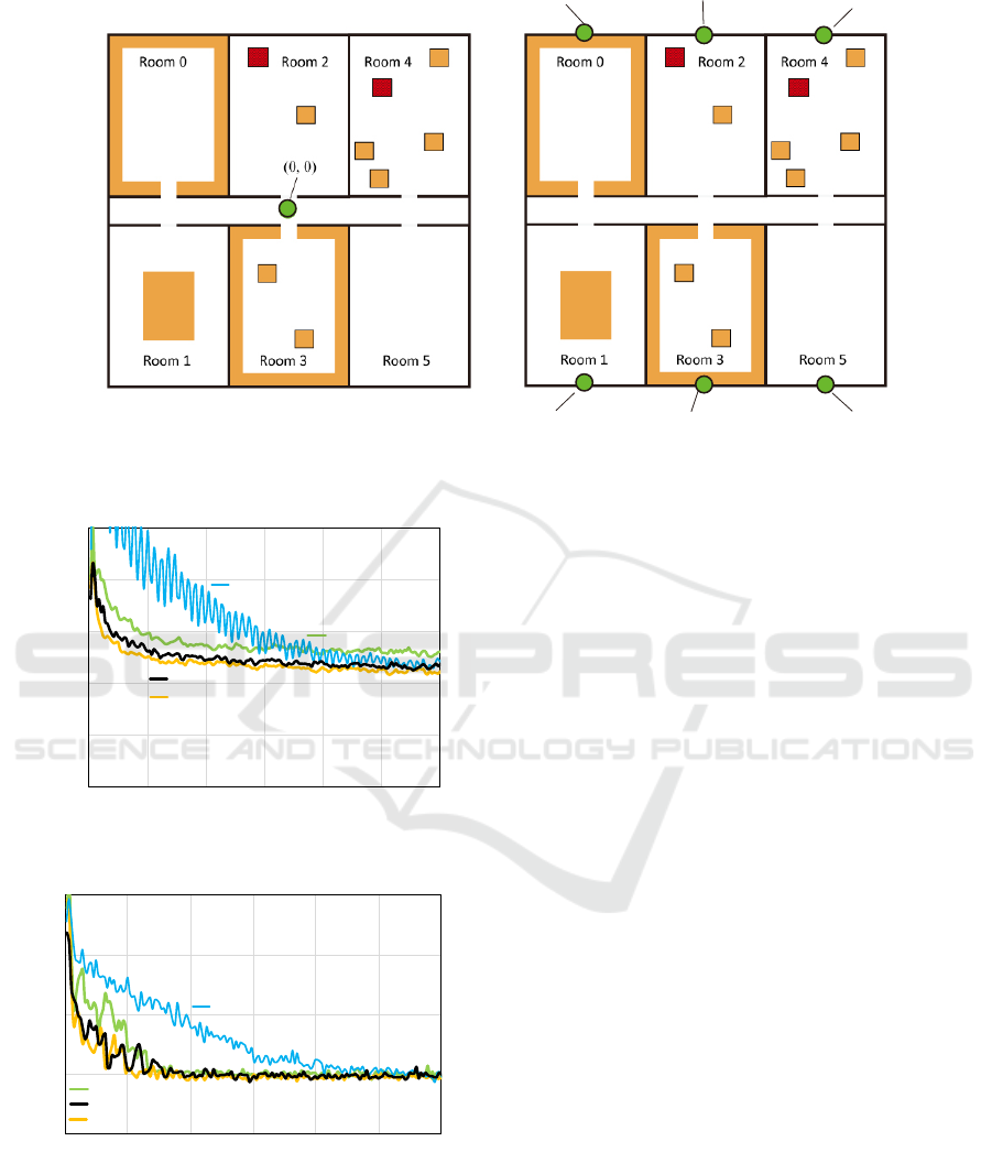
5.1 Experimental Setting

We constructed two simulated large environments,

called ”Ofﬁce A” and ”Ofﬁce B”, for agents to patrol

as shown in Fig. 1. These environments consisted of

six rooms (labeled Rooms 0-5), a corridor, and a num-

ber of nodes where events occurred frequently. We set

p(v) for v ∈ V as

p(v) =











−3

if v was in a red region,

−4

if v was in an orange region, and

−6

otherwise,

(14)

and the colored regions are shown in Fig. 1. The green

circles in these environments are charging bases. In

Ofﬁce A, all agents had charging bases in the same lo-

cation. In Ofﬁce B, we divided agents into six groups,

and the charging bases of each group were assigned to

one of six rooms differently. Each room had charging

bases in Ofﬁce B, but agents had to return to their own

assigned charging bases. The environments are repre-

sented by a 101 × 101 2-dimensional grid graph with

several obstacles (walls). We set the length of edges

between nodes to one.

We deployed 20 agents in the environments. We

assumed that agents did not know p

(v) in advance,

so we initially set p

(v) as 0. Agents started their

patrols from the assigned v

base

and periodically re-

turned to v

base

to recharge before their batteries be-

came empty. We set the actual battery speciﬁcations

of all agents as (B

max

drain

charge

) = (2700,1,3)

and set S

to S

= {300,900,2700}. When agents

selected s

to be 2700, the patrol cycle length was

maximum (10,800 ticks), whose breakdown consists

of the active time (2700 ticks) and the charging time

(8100 ticks). Therefore, for the target decision strat-

egy s we measured D

(s) and U

(s) every 14,400

ticks, which was longer than the maximum cycle

length. In experiments below, we set AMTDS/LD or

AMTDS/CL to s. The parameter values used in the

model are listed in Table 1.

5.2 Comparison of Fixed Activity Cycle

In the ﬁrst experiment, we compared the performance

results of four types of agents that used AMTDS/LD

with one of the ﬁxed ACLs, s

= 300, 900, or 2700

with those by the agents with AMTDS/CL in Ofﬁce A

as shown in Fig. 1(a). Hereinafter, AMTDS/LD with

ﬁxed ACL s

is denoted as AMTDS/LD(s

). The ex-

perimental results shown below are the average values

of ten independent experimental runs. Figure 2 plots

the performance, D(s), and Fig. 3 plots the perfor-

mance of U (s) over time. Note that the smaller D(s)

Learning of Activity Cycle Length based on Battery Limitation in Multi-agent Continuous Cooperative Patrol Problems

(-34, -50) (0, -50) (34, -50)

(-34, 50)

(0, 50)

(34, 50)

(b) Office B(a) Office A

Figure 1: Environments.

Figure 2: Improvement in D(s) over time in Ofﬁce A.

Figure 3: Improvement in U(s) over time in Ofﬁce A.

and U(s) are better.

Both ﬁgures indicate that agents with

AMTDS/LD(900) were the most efﬁcient, and

the agents with AMTDS/CL exhibited almost the

same efﬁciency as that with AMTDS/LD(900). The

efﬁciency of the agents with AMTDS/LD(2700) was

the worst and seemed unstable at ﬁrst, but it gradually

improved over time. Because AMTDS/LD(2700)

requires quite a long time to recharge, the num-

ber of patrolling agents were unstably ﬂuctuated.

However, the phases of their periodic cycles grad-

ually shifted naturally and ﬁnally disappeared. In

contrast, the converged performance of the agents

with AMTDS/LD(300) was always worse than the

others. This is because the ACL was too short to

cover the entire environment, especially areas distant

from the charging bases, and the agents in charge

of distant area had to return very frequently to the

charging bases. We can say that, in this particular

experimental environment, the ACL of 900 seemed

the best. However, this depends on the environmental

characteristics and we cannot decide the appropriate

ACL in advance. In comparison, the agents with the

proposed AMTDS/CL can adaptively select ACLs by

themselves without such a prior decision.

Figure 4 indicates the number of agents that se-

lected ∀s

∈ S

with AMTDS/CL over time. Note that

we plotted in this ﬁgure the values every 10,000 ticks

from 200,000 ticks; because agents started from de-

ciding the initial Q-values until 100,000 ticks and then

entered the learning of ACL from 100,000 ticks, the

learning results in the ﬁrst 200,000 were unstable. We

can see from this ﬁgure that many agents selected 900

ticks for s

since AMTDS/LD(900) exhibited the best

performance in this environment and this was consis-

tent with the results when agents have the ﬁxed ACL.

Additionally, we investigated the characteristics of

agents that selected 300 and 2700 as their ACL. Fig-

ICAART 2019 - 11th International Conference on Agents and Artiﬁcial Intelligence

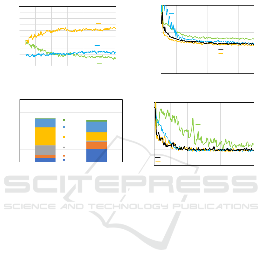
Figure 4: Number of agents selecting each s

over time in

Ofﬁce A.

50000

100000

150000

200000

250000

1 (selected 300 for s

c) 7 (selected 2700 for sc)

working me in each room (cks)

Agent ID

Room 0

Room 1

Room 2

Room 3

Room 4

Room 5

Figure 5: Working time in each Room of agent 1 and agent

7 in last 1,000,000 ticks in Ofﬁce A.

ure 5 shows the working time of agents whose IDs

were 1 and 7, i.e., how long they spent in each room

during the last 1,000,000 ticks. Note that Agent 1 se-

lected 300 and Agent 7 selected 2700 for their ACLs

at last, though 900 was usually the best as the ACL

in the environment. We also note that the data shown

in Fig. 5 is one result selected from the experimen-

tal trials, but we found that a similar tendency could

be observed in other trials. Agent 1 more often pa-

trolled Room 2 and Room 3 than Agent 7. Room 2

and Room 3 were near the charging base, Room 2 had

speciﬁc regions in which events frequently occurred,

and many nodes in Room 3 also had a higher p

(v).

Therefore, Agent 1 could ﬁnd many events in Room 2

and Room 3; thus, patrolling with a short ACL was

better from the viewpoint of Agent 1 to keep the num-

ber of unaware events low.

Meanwhile, Agent 7 frequently patrolled many

rooms, some of which were distant from the charg-

ing base. We conﬁrmed that, unlike Agent 1, Agent 7

had a high value of p

(v) in more and farther nodes,

so Agent 7 selected a long ACL to move around in a

large area. This analysis indicates that, from a global

viewpoint, agents with a short s

and long s

com-

plementarity covered different areas. That is because

some agents with AMTDS/CL did not select 900 for

Figure 6: Improvement in D(s) over time in Ofﬁce B.

Figure 7: Improvement in U(s) over time in Ofﬁce B.

and deterioration of efﬁciency was not occurred, al-

though AMTDS/LD(900) was best efﬁciency. These

results showed that agents with our method learned

the appropriate ACL s

without prior knowledge on

the environments, and actually, agents decided ACLs

on the basis of their learned p

(v) and working area.

We believe that such diversity in agent strategies also

enhances the response capabilities to environmental

changes as well as the improvement in the efﬁciency.

5.3 Adaptation to Environmental

Characteristics

In the second experiment, we also evaluated the four

types of agents in a slightly different environment

where there were six charging bases for each room,

named ”Ofﬁce B”, as shown in Fig. 1(b). A charg-

ing base in Room n is denoted by v

base-n

. We set

Agents 0, 1, 2, and 3 to v

base-0

, Agents 4, 5, and 6

to v

base-1

, Agents 7, 8, and 9 to v

base-2

, Agents 10, 11,

12, and 13 to v

base-3

, Agents 14, 15, and 16 to v

base-4

and Agents 17, 18, and 19 to v

base-5

. The improve-

ment D(s) is plotted in Fig. 6, and U(s) over time in

Ofﬁce B is plotted in Fig. 7.

We can conﬁrm that the efﬁciency of AMTDS/CL

and AMTDS/LD(900) was almost identical from

Learning of Activity Cycle Length based on Battery Limitation in Multi-agent Continuous Cooperative Patrol Problems

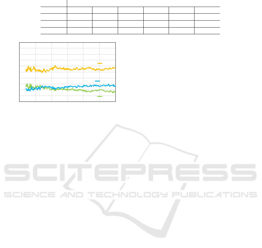
Table 2: Number of agents selecting each s

described by their charging bases at 3,000,000 tick in Ofﬁce B.

Location of charging base

Room 0 Room 1 Room 2 Room 3 Room 4 Room 5

=300 1.2 0.3 0.2 1.7 0.0 0.0

=900 2.1 1.7 2.3 2.2 2.1 1.0

=2700 0.7 1.0 0.5 0.1 0.9 2.0

Figure 8: Number of agents selecting each s

over time in

Ofﬁce B.

these ﬁgures. If we carefully compare Fig. 6 with

Fig. 2, the converged performances of all methods

were almost identical in both performances. How-

ever, the convergence of the AMTDS/LD(2700) in

Fig. 6 seemed faster, and the performance also

seemed stabler than those of AMTDS/LD(2700) in

Fig. 2. In Ofﬁce B, the charging bases were dis-

tributed, so the patrol patterns of individual agents

differed even if agents had the same length of ACL.

Figure 7 indicates that agents with AMTDS/LD(300)

were the worst, which differed from the results of

the ﬁrst experiment (see Fig. 3). This indicates that

the performance, U(s), also depended on the distance

between the charging bases and the work locations.

In the second experiment, the areas individual agents

visited were distinct, so nodes were covered by a

smaller number of agents than in Ofﬁce A.

The number of agents that selected each s

for

AMTDS/CL as shown in Fig. 8, was similar charac-

teristic to Fig. 4. In this experiment, we were inter-

ested in the differences in ACL learned on the basis of

the locations of agents’ charging bases. Table 2 lists

the average number of agents that selected s

∈ S

for

AMTDS/CL for each charging base location. This ta-

ble shows that 900 was mainly selected as the value of

by many agents, but we can observe different char-

acteristics according to agents’ base locations. We

already knew that 900 was appropriate for this en-

vironment; thereby, we focused on and analyzed the

agents that selected other ACLs. Agents whose charg-

ing base was in Room 5 obviously learned that the

long ACLs were better. Because they could ﬁnd only

a few events near their base (Room 5 did not have

a node with a high p(v)), they had to explore nodes

farther away to help other agents. Relatively more

agents whose bases were in Rooms 0 and 3 selected

300 as their ACL. In these rooms, there were many

nodes with a high p(v) as shown in Fig. 1. Thus,

these agents could ﬁnd many events near their bases.

By selecting the shorter ACLs, they could reduce the

cost of moving to other rooms and focused on speciﬁc

nodes in the local rooms. In addition, they could visit

nearby nodes at an appropriate and shorter frequency

by improving the accuracy of the estimated p

(v) for

the speciﬁc nodes.

When we carefully observed the experimental

runs, we found that agents whose base was in Room 5

selected 900 as their ACL at ﬁrst, but after that, they

gradually changed to 2700. We can explain this

change as follows. At ﬁrst, they selected 900 since

it seemed more appropriate than others. However, af-

ter other agents whose bases were in other rooms fo-

cused on nodes near their base and improved their pa-

trol performance. In contrast, there were no nodes

with high importance values p

(v) in Room 5, and

agents whose base was Room 5 had to visit more of

the other rooms to ﬁnd events. This suggests indi-

rect communication through learning the importance

value. Therefore, agents could perform well by learn-

ing the ACLs to improve the entire system perfor-

mance in a real-time manner, and this learning of the

length was thanks to the results of the learning of im-

portance p

(v).

6 CONCLUSION

We proposed an autonomous method for learning

the activity cycle length, which is how long indi-

vidual agents act to work in collaborative environ-

ments. This method reﬂects the activities of other

collaborative agents, which are also learning mutu-

ally to contribute to the entire performance. We ex-

perimentally showed that agents with our method,

AMTDS/CL, performed effectively comparable with

the same efﬁciency as the best case with a ﬁxed ACL,

without giving any prior knowledge on the best ACL

and the environmental characteristics in advance. We

also analyzed the relationships between the selected

ACL and agents’ behaviors. Nodes were covered

ICAART 2019 - 11th International Conference on Agents and Artiﬁcial Intelligence

with a number of agents with different frequencies,

phases, and periods; this resulted in effective cover-

ing of the environment only through lightweight com-

munication with others. We also proposed a strategy

in which agents select the appropriate activity cycle

length from among ﬁxed possible activity cycles be-

cause we think that agents have to consider complex-

ity to estimate the environmental workload.

Our future work is to ﬁnd an activity control strat-

egy in which agents estimate a workload with high

accuracy and ﬂexibility to control their activity while

taking into account their remaining energy.

ACKNOWLEDGMENT

This work was partly supported by JSPS KAKENHI

Grant Number 17KT0044 and Grant-in-Aid for JSPS

Research Fellow (JP16J11980).

REFERENCES

Ahmadi, M. and Stone, P. (2006). A multi-robot system for

continuous area sweeping tasks. In Proceedings of the

2006 IEEE International Conference on Robotics and

Automation, pages 1724 – 1729.

Bentz, W. and Panagou, D. (2016). An energy-aware re-

distribution method for multi-agent dynamic coverage

networks. In 2016 IEEE 55th Conference on Decision

and Control (CDC), pages 2644–2651.

Chen, X. and Yum, T. P. (2010). Patrol districting and rout-

ing with security level functions. In 2010 IEEE Inter-

national Conference on Systems, Man and Cybernet-

ics, pages 3555–3562.

Chevaleyre, Y. (2005). Theoretical analysis of the multi-

agent patrolling problem. In Proceedings of Intelligent

Agent Technology, pages 302–308.

David, P. and Rui, R. (2011). A survey on multi-robot pa-

trolling algorithms. In Camarinha-Matos, L. M., edi-

tor, Technological Innovation for Sustainability: Sec-

ond IFIP WG 5.5/SOCOLNET Doctoral Conference

on Computing, Electrical and Industrial Systems, Do-

CEIS 2011, Costa de Caparica, Portugal, February

21-23, 2011. Proceedings, pages 139–146. Springer

Berlin Heidelberg.

Jensen, E., Franklin, M., Lahr, S., and Gini, M. (2011).

Sustainable multi-robot patrol of an open polyline. In

2011 IEEE International Conference on Robotics and

Automation, pages 4792–4797.

Machado, A., Ramalho, G., Zucker, J.-D., and Drogoul, A.

(2003). Multi-agent patrolling: An empirical analy-

sis of alternative architectures. In Sim

ao Sichman, J.,

Bousquet, F., and Davidsson, P., editors, Multi-Agent-

Based Simulation II, pages 155–170, Berlin, Heidel-

berg. Springer Berlin Heidelberg.

Pasqualetti, F., Durham, J. W., and Bullo, F. (2012). Co-

operative patrolling via weighted tours: Performance

analysis and distributed algorithms. IEEE Transac-

tions on Robotics, 28(5):1181–1188.

Popescu, M. I., Rivano, H., and Simonin, O. (2016). Multi-

robot patrolling in wireless sensor networks using

bounded cycle coverage. In 2016 IEEE 28th Interna-

tional Conference on Tools with Artiﬁcial Intelligence

(ICTAI), pages 169–176.

Santana, H., Ramalho, G., Corruble, V., and Ratitch, B.

(2004). Multi-agent patrolling with reinforcement

learning. In Proceedings of the Third International

Joint Conference on Autonomous Agents and Multia-

gent Systems - Volume 3, AAMAS ’04, pages 1122–

1129, Washington, DC, USA. IEEE Computer Soci-

ety.

Sipahioglu, A., Kirlik, G., Parlaktuna, O., and Yazici, A.

(2010). Energy constrained multi-robot sensor-based

coverage path planning using capacitated arc routing

approach. Robot. Auton. Syst., 58(5):529–538.

Sugiyama, A., Sea, V., and Sugawara, T. (2016). Effective

task allocation by enhancing divisional cooperation in

multi-agent continuous patrolling tasks. In 2016 IEEE

28th International Conference on Tools with Artiﬁcial

Intelligence (ICTAI), pages 33–40.

Sugiyama, A. and Sugawara, T. (2017). Improvement of

robustness to environmental changes by autonomous

divisional cooperation in multi-agent cooperative pa-

trol problem. In Demazeau, Y., Davidsson, P., Bajo,

J., and Vale, Z., editors, Advances in Practical Appli-

cations of Cyber-Physical Multi-Agent Systems: The

PAAMS Collection, pages 259–271, Cham. Springer

International Publishing.

Yoneda, K., Kato, C., and Sugawara, T. (2013). Au-

tonomous learning of target decision strategies

without communications for continuous coordinated

cleaning tasks. In Web Intelligence (WI) and Intelli-

gent Agent Technologies (IAT), 2013 IEEE/WIC/ACM

International Joint Conferences on, volume 2, pages

216–223.

Learning of Activity Cycle Length based on Battery Limitation in Multi-agent Continuous Cooperative Patrol Problems