Bayesian Optimization of 3D Feature Parameters for 6D Pose Estimation

Frederik Hagelskjær, Norbert Kr

uger and Anders Glent Buch

Maersk Mc-Kinney Moller Institute, University of Southern Denmark, Odense, Denmark

Keywords:

Pose Estimation, Object Detection, Feature Matching, Optimization, Bayesian Optimization, Machine

Learning.

Abstract:

6D pose estimation using local features has shown state-of-the-art performance for object recognition and pose

estimation from 3D data in a number of benchmarks. However, this method requires extensive knowledge

and elaborate parameter tuning to obtain optimal performances. In this paper, we propose an optimization

method able to determine feature parameters automatically, providing improved point matches to a robust

pose estimation algorithm. Using labeled data, our method measures the performance of the current parameter

setting using a scoring function based on both true and false positive detections. Combined with a Bayesian

optimization strategy, we achieve automatic tuning using few labeled examples. Experiments were performed

on two recent RGB-D benchmark datasets. The results show signiﬁcant improvements by tuning an existing

algorithm, with state-of-art performance.

1 INTRODUCTION

Pose estimation is the task of determining the position

and orientation of one or multiple objects in a scene,

e.g. as seen in Fig. 1. The scene data could be either

2D or 3D data coming from one or multiple sensors.

A wide range of new sensors, with the Kinect (Zhang,

2012) at the forefront, has enabled easy access to 3D

data. This has resulted in 3D feature matching as a vi-

able tool for pose estimation. The pose is represented

by a transformation matrix consisting of a translation

and rotation, which can be passed on for further use,

e.g. during robotic grasping.

A widely used method for addressing the task of

pose estimation in 3D data is feature matching using

local shape descriptors. This method goes back 20

years with the well-known Spin Images (Johnson and

Hebert, 1999) and has become the de facto standard

for 3D pose estimation (Guo et al., 2014). Matches

between object and scene points are found in feature

space and are used to ﬁnd the transform between the

to point clouds. This approach is especially suitable

for scenarios where parts of the object are occluded,

as the matching is performed locally. Many different

features have been developed, e.g. SHOT (Salti et al.,

2014), FPFH (Rusu et al., 2009), and USC (Tombari

et al., 2010). A fundamental limitation when applying

such descriptors is that the performance depends he-

avily on careful parameter tuning, the size of the lo-

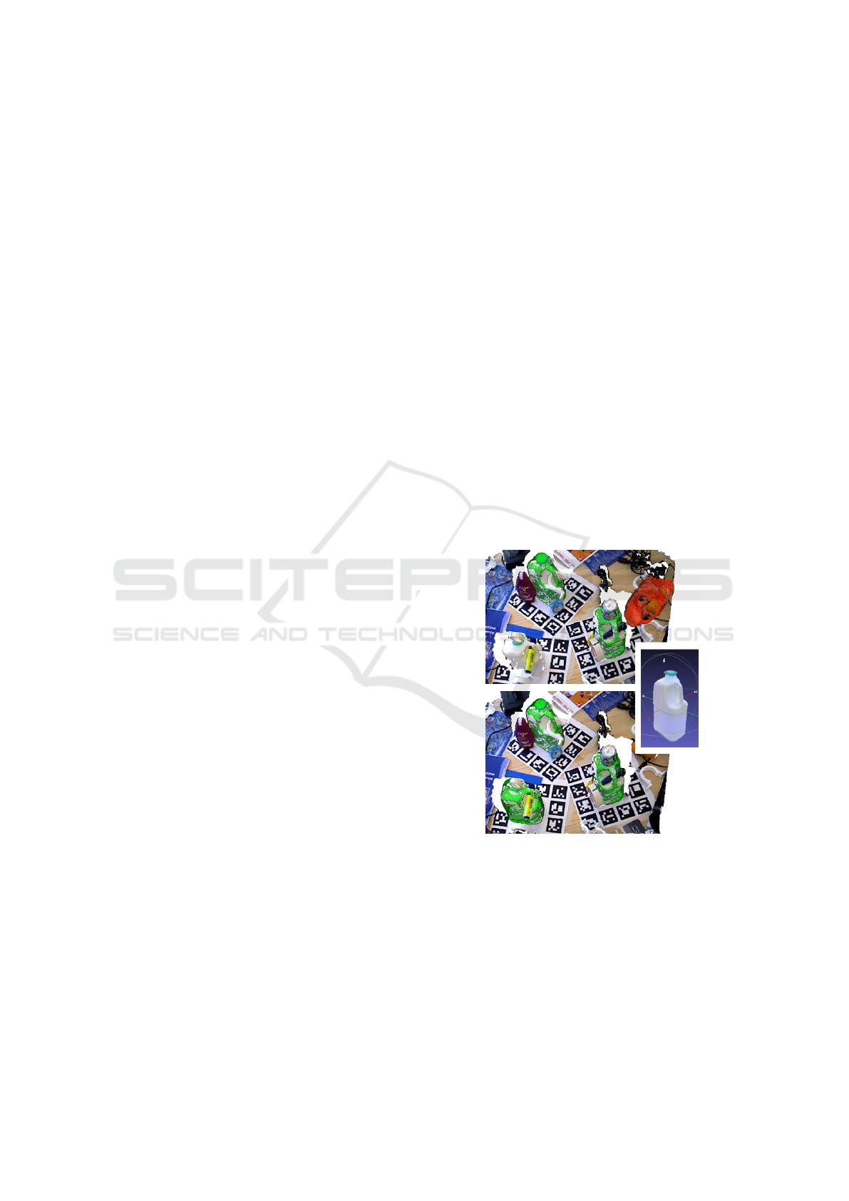
Figure 1: Multi-instance pose estimation example for a

scene from the dataset of (Tejani et al., 2014). To the top is

shown an example with non-optimized feature parameters,

resulting in two correct (green) and one incorrect detection

(red). The CAD model of the object is shown in the middle.

Our parameter optimization improves the pose estimation

algorithm, giving correct detection of all the three instances

of the object shown at the bottom.

cal support radius is shown to be extremely important

(Guo et al., 2016), which must be set to a compromise

between descriptive power and occlusion tolerance.

If set incorrectly, the matching will perform badly

Hagelskjær, F., Krüger, N. and Buch, A.

Bayesian Optimization of 3D Feature Parameters for 6D Pose Estimation.

DOI: 10.5220/0007568801350142

In Proceedings of the 14th International Joint Conference on Computer Vision, Imaging and Computer Graphics Theory and Applications (VISIGRAPP 2019), pages 135-142

ISBN: 978-989-758-354-4

135

Figure 2: Full pipeline of our parameter optimization approach. ’p’ training scenes are selected and for each scene ’m’

objects are present. Resulting in m*p object detections. A: First a parameter set is used for object recognition. B: The scoring

function then determines the performance. C: The Gaussian Process ﬁts a distribution to the results. D: The decision selects

the next parameters sets to test. A number of preselected parameter sets are used to build the Gaussian Process, after which the

Bayesian Optimization runs for n-iterations. E: the full set of parameters and scores is ﬁt to an additional Gaussian Process

and the expected best parameter set is found F.

and so will the pose estimation algorithm, which uses

these matches for the sampling process.

In a comparison of different features, this varia-

bility is shown as an error greatly inﬂuencing perfor-

mance (Guo et al., 2016). And in papers presenting

the performance of new features the tuning is done by

the author who searches for the best performance, and

leaves out all other results. We believe the parameter

values to be fundamental in the feature matching task

and propose a systematic approach to choosing the

best parameters.

Although the data-driven approach for object re-

cognition for 3D data is old (Oshima and Shirai,

1983), the knowledge-driven ﬁne tuning is the one of-

ten seen in benchmarking. In this paper we focus on

the data-driven approach. Scenes are split into a trai-

ning and test set, but compared to modern approaches

towards 3D tasks, e.g. (Qi et al., 2017), we also show

good results with much smaller training samples. Ad-

ditionally, we employ Bayesian Optimization (Snoek

et al., 2012) to search the parameter space. But as we

are only searching a small dataset, instead of using

a single maximum value we ﬁt a Gaussian process

(Rasmussen, 2004) to the results to avoid local maxi-

mums. An overview of the full method can be seen in

Fig. 2.

In a study of the usage of pose estimation, the me-

dian time to setup a system was found to be between

1–2 weeks (Hagelskjær et al., 2017), with most of

the work being done on the software side. To enable

an easier use of object recognition in real applicati-

ons, automatic optimization approaches can be help-

ful. This paper presents a principled method for doing

so, with a focus on some of the most important para-

meters for local shape descriptor computation. Our

method, however, can be applied in a wide range of

applications.

The remaining article is structured as follows:

Section 2 outlines the methods used for pose estima-

tion along with other optimization approaches. Our

method is presented in Section 3. Section 4 contains

experimental results of our method compared with

current methods. Finally, we outline the conclusion

of our work and the further perspectives of this ap-

proach.

2 PROPOSED METHOD

Parameter tuning using Bayesian Optimization has

begun to be widely used in machine learning. Despite

this, to the best of our knowledge, automatic parame-

ter tuning has not yet been seen for 3D feature des-

criptors. Although e.g. (Jørgensen et al., 2018) cover

optimal camera placements in a robotic setup, it does

not go into the parameters of feature matching. We

start by outlining the feature matching for pose esti-

mation task, then we outline the Bayesian Optimiza-

tion method and ﬁnally we describe how it is used to

tune parameters.

2.1 Pose Estimation with Feature

Matching

Pose estimation based object recognition is the task

of determining the position of one or multiple ob-

jects in a scene. A typical strategy towards a solu-

tion to this problem is to represent the scene by a

2D image, wherein template matching of object views

are performed (Hinterstoisser et al., 2012). This ap-

proach, however, is not well suited to handle occlusi-

VISAPP 2019 - 14th International Conference on Computer Vision Theory and Applications

136

Figure 3: The important descriptor parameters for a single point in a point cloud. To the left is shown a representation of

parameters: For each point, the Normal Radius is used to select nearby points for calculating the normal vector. All points

within the Keypoint Radius is then used to compute the descriptor. In the middle the size of feature radius is shown, the 30

mm represent 10 % of the object size. To the right is shown a 10 mm normal radius, zoomed.

ons of the object. Feature based methods such as e.g.

SIFT (Lowe, 1999) were developed, which describe

local patches. At roughly the same time, new descrip-

tors were also developed for 3D data, e.g. the Spin

Image descriptor(Johnson and Hebert, 1999). The

Spin image is a local descriptor based on the idea of

an object-centered viewpoint. In the 2D case the lo-

cal descriptor is calculated with orientation towards

the camera, as the geometry is unknown. In the 3D

case the normal vector at the point can be calculated

and instead of using the coordinate system of the ca-

mera, a local coordinate system is found. This makes

the descriptor much more robust to both translation

and rotation in depth (Hagelskjaer et al., 2017). The

object-centered viewpoint is used for many of the fol-

lowing descriptors which have later been developed.

The Spin Image encodes the number of points that fall

into nearby spatial bins, relative to the surface point

being described. This use of relational information

has been used in many following descriptors, for in-

stance SHOT (Salti et al., 2014), FPFH (Rusu et al.,

2009), and USC (Tombari et al., 2010), to name a few.

In this work we use local shape descriptor which col-

lects four simple relations for each point in the spher-

ical neighborhood around the point to be described.

These relations are taken from the point pair feature

(PPF) (Drost et al., 2010) and rely on the computation

of surface normals, similar to the majority of other

shape descriptors available. The relations are binned

into a number of histograms, which together describe

the local shape variation. This descriptor has been

successfully used earlier for pose estimation and ob-

ject recognition tasks (Buch et al., 2017). An illus-

tration of the computation of the PPF based feature

in a scene with corresponding parameters is shown in

Fig. 3. Using training-data for pose estimation have

also been performed using deep learning (Kehl et al.,

2017; Rad and Lepetit, 2017; Do et al., 2018). These

approaches show impressive performance, but have a

number of limitations. The trained network is a com-

plex model with many parameters requiring a large

amount of well representing data. This restricts the

setup of new systems as training data needs to either

collected or generated. These methods expects the ob-

ject standing on a table and have not been tested on the

bin-picking dataset. Compared to this our approach is

based on methods only requiring a CAD model.

2.2 Optimization Strategy

In the previous section the importance of choosing

correct values for shape descriptor parameters where

highlighted. It is, therefore, necessary to explore the

parameter space and obtain an optimum conﬁguration

according to some criterion. An exhaustive search of

the full parameter space is intractable, thus it is desi-

rable to derive a proper search strategy.

2.2.1 Optimization Algorithms

Optimization algorithms in general is a widely stu-

died subject, and a number of different methods exist.

One of the more straightforward approaches is gra-

dient descent wherein the gradient of the loss function

is used to update the parameter setting. Thus, given

a starting point, the parameters are gradually updated

until a maximum is found. This also has the advan-

tage that it can be easily speciﬁed when to terminate

the optimization. For the pose estimation problem

two difﬁculties for gradient descent arise. First, the

loss function cannot be expected to be either smooth

or convex. Fundamentally, the score is the number of

correct detections, which is a subset of the list of natu-

ral numbers N. The gradient of this function cannot be

expected to be non zero. As a limited number of sce-

nes are used for our purposes, the score function will

be expected to ﬂuctuate. It is, therefore, necessary

to perform non-smooth non-convex optimization, for

which many different methods have been developed

(Rios and Sahinidis, 2013).

Bayesian Optimization of 3D Feature Parameters for 6D Pose Estimation

137

(a) Score for different para-

meters set run on the training

data.

(b) The resulting mean of the

ﬁtted Gaussian Process.

the ﬁtted Gaussian Process.

(d) The Upper Conﬁdence

Bound plot by combining

mean and variance.

Figure 4: Loop of a single bayesian optimization. Notice the variance is zero at each data point. The next iteration will be at

the highest point in the Upper Conﬁdence Bound plot.

2.2.2 Bayesian Optimization

We decided to use Bayesian optimization, a method

for bounded global optimization (Snoek et al., 2012).

Bayesian optimization has been employed success-

fully for tuning machine learning parameters as well

as many other applications (Bergstra et al., 2013), and

an implementation is readily available (Snoek et al.,

2012). Bayesian optimization is also a good approach

when evaluations are expensive as is the case of pose

estimation. Benchmarking of optimization algorithms

have shown Bayesian Optimization with state-of-art

performance(Jones, 2001). Compared with other non-

gradient methods, i.e. evolutionary algorithms and

particle ﬁlters Bayesian Optimization use qualiﬁed

guesses and not random mutations and sampling and

thus requires fewer iterations.

In Bayesian optimization all previous samples are

used to ﬁt a surrogate model and using this surro-

gate model the next sample to evaluate is selected.

A number of initial samples are made using random

uniform sampling within the bounds for the parame-

ters. The used surrogate model is a Gaussian process

(Rasmussen, 2004), a non-parametric method which

utilizes all previous samples to create the model. Ad-

ditionally, the Gaussian process also provides a pro-

bability of the prediction. The well-known Upper

Conﬁdence Bound (UCB) is used as the acquisition

function (Snoek et al., 2012). As the name implies the

conﬁdence bound over the current maximum is used

to select the next parameter setting to investigate. An

illustration of the a single step in the Bayesian opti-

mization can be seen in Fig. 4.

2.3 Our Approach

The pose estimation system we optimize is based on

the voting approach presented in (Buch et al., 2017).

This algorithm is freely available online

and direct

comparison can be performed with existing results.

https:://www.gitlab.com/caro-sdu/covis

We decide to optimize the size of the feature radius

and the normal radius, as these parameters are fun-

damental to all feature matching algorithms and are

easily understood. The goal of our approach is to ﬁnd

the parameter set which gives the best performance

for pose estimation. For the datasets used in this work,

recall and maximum F1-score were used (Hinterstois-

ser et al., 2012; Tejani et al., 2014) to evaluate perfor-

mance of a recognition system. Recall is deﬁned as

the number of correct detections found from the full

dataset. A detection is deﬁned as correct if the transla-

tion distance is less than 50 mm and the angular error

for the Z-axis is less than 15

◦

. F1-score is deﬁned as a

combination of both recall and precision, where preci-

sion is the number of correct detections to the number

of returned detections.

2.3.1 Scoring the Detections

To optimize for stable detections, we utilize the score

given from the detection algorithm to create a new

score for the optimization system. We split the sco-

res given by the system into correct (true positives,

TPs) and wrong detections (false positives, FPs), thus

getting respectively KDE

T P

and KDE

. The KDE

is the output kernel density score for a pose pro-

vided by the underlying pose voting method (Buch

et al., 2017) used for the estimation, but any scoring

function could in principle be used here. We then use

the TP/FP ratio as the score, as seen in (1), penalizing

has high scores for wrong detections and rewarding

high scores for correct detections. The score function

is log-transformed for numerical reasons, as this leads

to more stable performance when invoking the opti-

mization algorithm.

score(KDE)

(

log(

∑

KDE

T P

∑

KDE

), if

∑

KDE

T P

≥

∑

KDE

0, otherwise

(1)

VISAPP 2019 - 14th International Conference on Computer Vision Theory and Applications

138

Figure 5: Result of ﬁtting a Gaussian process to the samples from the Bayesian optimization. The best parameter set is then

found by the maximum position of the resulting ﬁt.

2.3.2 Gaussian Process Regression for Mode

Finding

As only a small training set is used, there is a risk

of overﬁtting the parameters to only the particular set

of training scenes seen during training. To decrease

the risk of wrong parameters we additionally employ

a Gaussian Process to regress over the ﬁnished set of

evaluations, which is then used to predict the best pa-

rameter set in a more smooth and robust manner.

Other approaches have also been made to

avoid overﬁtting Bayesian optimization techniques to

sparse training sets. In (Dai Nguyen et al., 2017) a

term is added to the acquisition function which pe-

nalizes sharp peaks. In our approach we focus on ex-

ploration, but use the classical Bayesian optimization,

and then ﬁt all explored points with a Gaussian Pro-

cess to determine a stable maximum. The number of

explored points, n, can be described as the matrix con-

sisting of the parameters X and the resulting score y.

X, y = {(x

, f (x

) ) | i = 1, ..., n} (2)

To predict the expected score at new parameter va-

lues with a Gaussian Process, a distribution is requi-

red. Here ˆx is denoting a new untested parameter set.



ˆx



∼



K K

ˆx

ˆx ˆx



(3)

Where K is a covariance matrix given by a se-

lected kernel, k(x

, x

), wherein each index is calcu-

lated by the relationship of two parameter sets. This

gives that K

nxn

, K

nx1

and K

ˆx ˆx

. We are now able to

ﬁnd the expected value of the new parameter set by

the mean and the uncertainty as the variance (Ebden,

2008).

E( ˆx) = K

ˆx

−1

y (4)

var( ˆx) = K

ˆx ˆx

− K

ˆx

−1

ˆx

(5)

To make the Gaussian process more stable to

noise, a second term is added to the covariance

function, compared with the Bayesian Optimization

(Snoek et al., 2012), giving a Matern-kernel and a

White Noise kernel, as shown in (6). Here the ker-

nel function K takes distance d as input, combining

the Matern covariance C

and a diagonal noise term

K(d) = C

(d) + N(d) (6)

Γ and J denote the gamma function and the Bessel

function, respectively. The white noise (8) adds the

uncertainties in the evaluation as the full dataset is not

used. An illustration of a 2D regression can be seen

in Fig. 5, representing the scores for parameters sets

trained the training images shown in Fig. 6.

(d) = σ

1−ν

Γ(ν)



√

2ν





√

2ν



(7)

N(d) =

(

σ, if d = 0

0, otherwise

(8)

This kernel is used create the covariance matrices,

but before the prediction can be calculated, parame-

ters for (7) and (8) needs to be determined. A minimi-

zation using (Byrd et al., 1995) is performed that ﬁts

the parameter values to the known score y while ﬁx-

ing the ν value, i.e. how much distant points interact

with predicted result. This is to ensure a more smooth

prediction of parameters. With these values the kernel

can be calculated and a more robust function for the

expected parameter space can be created.

Using the training data and the scoring system the

parameter space is explored using Bayesian optimi-

zation and a number of samples are collected. These

samples are then used to ﬁt a Gaussian process as seen

in (6) from which a maximum parameter set is found.

Bayesian Optimization of 3D Feature Parameters for 6D Pose Estimation

139

Table 1: Results for the tabletop dataset (Tejani et al., 2014). All results are given as F1 scores.

Method Camera Coffee Joystick Juice Milk Shampoo Avg

(Doumanoglou et al., 2016) 0.903 0.932 0.924 0.819 0.510 0.735 0.803

(Kehl et al., 2017) 0.603 0.991 0.937 0.977 0.954 0.859 0.856

(Li and Hashimoto, 2018) 0.741 0.983 0.997 0.919 0.780 0.999 0.910

Org (Buch et al., 2017) 0.711 0.993 0.973 0.975 0.776 0.709 0.856

Ours 0.853 0.999 0.994 0.973 0.859 0.796 0.912

3 EXPERIMENTS

We ran extensive evaluations on two commonly used

RGB-D based object recognition datasets. The ﬁrst

dataset of Tejani et al. (Tejani et al., 2014) contains

six tabletop sequences for multi-instance pose estima-

tion (see Fig. 1 for an example). The scenes contain

large amounts of cluttering and background structu-

res. The second dataset of Doumanoglou et al. (Dou-

manoglou et al., 2016) contains two objects (a coffee

cup and a juice box) and three test sequences, all sho-

wing multiple instances of the objects in a bin. There

is a dedicated sequence per object and a mixed se-

quence, where both objects appear in the bin.

3.1 Selection of Training Images

The tested datasets unfortunately do not have training

scenes, which required us to take some out for trai-

ning. In (Brachmann et al., 2016) a scheme for se-

lecting training data in already existing datasets have

been proposed. This scheme has been reused in a

number of papers (Rad and Lepetit, 2017; Tekin et al.,

2018). This approach samples the full range of poses

in the dataset by adding all images that deviate more

than 15 degrees from images already in the training

set. An example of the difference between each trai-

ning image is shown in Fig. 6. As this would cover

33 percent of the dataset for the bin picking dataset a

different approach is chosen in this article.

From each dataset, we collected eight random sce-

nes for training, considerable less than the more than

100 used in (Brachmann et al., 2016; Rad and Lepetit,

2017; Tekin et al., 2018).

For our optimization, ten initial parameter sam-

ples drawn uniformly in space and 25 subsequent ite-

rations were made using Bayesian optimization with

our KDE scoring. Lastly the Gaussian process regres-

sion model was ﬁtted and a maximum was calculated.

A speciﬁc example can be seen in Fig. 1, where our

method enable successful recognition of all three in-

stances of a model in a scene from the tabletop data-

set.

3.2 Results

Comparison was done with the original pose voting

method (Buch et al., 2017) and for the tabletop data-

set we included the current state of the art (Doumano-

glou et al., 2016; Li and Hashimoto, 2018) from the

literature. Compared with the original pose voting al-

gorithm, we obtain a 7% increase in performance on

the tabletop scenes on average (second column from

the right). Interestingly, our optimization also allows

the pose voting method to surpass state of the art on

this dataset. For completeness, we have additionally

included a rightmost column where we do not include

the eight training scenes in the testing to show that

this causes a marginal difference in results.

For the bin picking dataset (Doumanoglou et al.,

2016) no current method seems to outperform (Buch

et al., 2017), we decided to include two other known

methods to show not only compare with the original

approach. The results can be seen in Tab. 2. Here we

substantially outperform the baseline on average, but

perform slightly worse on the coffee cup. We believe

this is because the performance on this object close to

saturated already, with the chosen parameters.

Table 2: Results for bin picking dataset (Doumanoglou

et al., 2016). All results are given as recall rates, as per

the protocol for this dataset.

Method Coff Juice Avg.

(Tejani et al., 2014) 31.4 24.8 28.1

(Doumanoglou et al., 2016) 36.1 29.0 32.6

Org (Buch et al., 2017) 63.8 44.9 54.4

Ours 63.4 51.7 57.6

3.3 Sensitivity to the Number of

Training Images

We also wanted to test the ability of our method to

generalize to the test set using a varying number of

training scenes. This experiment was performed on

the bin picking dataset. It is clear from Fig. 7 that the

number of scenes is important for the resulting per-

formance. As the number of scenes increases, so does

the performance in general, although eight scenes in

VISAPP 2019 - 14th International Conference on Computer Vision Theory and Applications

140

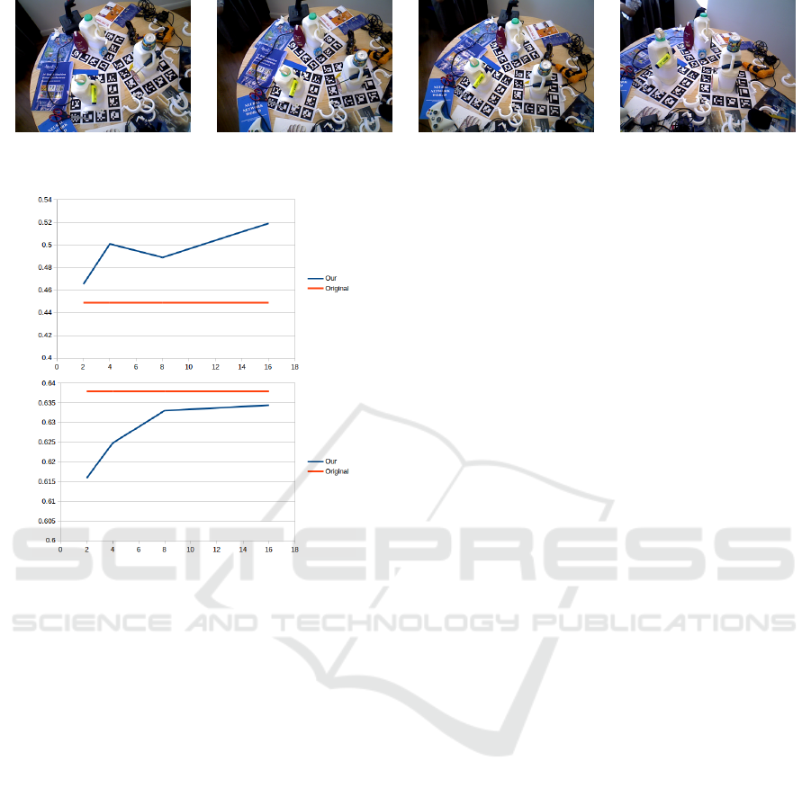
Figure 6: Sequence of the ﬁrst four images used for the training of object ”05” of the Tejani dataset. There is atleast a 15

degree angle between each object.

Figure 7: Results of ﬁtting a Gaussian process to increasing

training set sizes from the bin picking dataset. To the left

is shown the result of varying the number of training scenes

for the juice, and to the right the same for the coffee cup.

the juice dataset gives a drop. This is likely from an

unfortunate random sample of a subset of scenes that

do not properly represent the full data. For the coffee

cup dataset the performance is slightly increasing as

more samples are added, although it is still not able

to outperform the original. A 1 dimensional grid se-

arch was performed on the full dataset which shows

that the original performance is actually at the best

possible and all our found parameter sets are circling

around this performance.

4 CONCLUSIONS

In this work we have demonstrated the feasibility

of using Bayesian optimization in combination with

Gaussian Process regression for automatically deter-

mining optimal parameters for an existing 3D shape

descriptor based object recognition and pose estima-

tion system. Our method is useful for bounded global

optimization within a chosen parameter space that is

crucial to the performance of the method that is to

be tuned. We have demonstrated our approach on a

recent pose estimation algorithm, optimizing two of

the most important hyper-parameters for the descrip-

tor calculation process.

Our method is able to signiﬁcantly improve the

performance on the chosen pose estimation algorithm,

providing improved results compared to state the art

algorithms on two RGB-D datasets. We see our met-

hod as more generally applicable for optimization of

many other parameters than the two descriptor pa-

rameters used in this work. We will pursue this di-

rection for future work.

ACKNOWLEDGEMENTS

This work has been supported by the H2020 project

ReconCell (H2020-FoF-680431).

REFERENCES

Bergstra, J., Yamins, D., and Cox, D. D. (2013). Making

a science of model search: Hyperparameter optimiza-

tion in hundreds of dimensions for vision architectu-

res. Journal of Machine Learning Research.

Brachmann, E., Michel, F., Krull, A., Ying Yang, M., Gum-

hold, S., et al. (2016). Uncertainty-driven 6d pose esti-

mation of objects and scenes from a single rgb image.

In Proceedings of the IEEE Conference on Computer

Vision and Pattern Recognition, pages 3364–3372.

Buch, A. G., Kiforenko, L., and Kraft, D. (2017). Rota-

tional subgroup voting and pose clustering for robust

3d object recognition. In International Conference on

Computer Vision (ICCV).

Byrd, R. H., Lu, P., Nocedal, J., and Zhu, C. (1995). A

limited memory algorithm for bound constrained op-

timization. SIAM Journal on Scientiﬁc Computing,

16(5):1190–1208.

Dai Nguyen, T., Gupta, S., Rana, S., and Venkatesh, S.

(2017). Stable bayesian optimization. In Paciﬁc-Asia

Conference on Knowledge Discovery and Data Mi-

ning, pages 578–591.

Do, T.-T., Cai, M., Pham, T., and Reid, I. (2018). Deep-

6dpose: Recovering 6d object pose from a single rgb

image. arXiv preprint arXiv:1802.10367.

Bayesian Optimization of 3D Feature Parameters for 6D Pose Estimation

141

Doumanoglou, A., Kouskouridas, R., Malassiotis, S., and

Kim, T.-K. (2016). Recovering 6d object pose and

predicting next-best-view in the crowd. In Internati-

onal Conference on Computer Vision and Pattern Re-

cognition (CVPR), pages 3583–3592.

Drost, B., Ulrich, M., Navab, N., and Ilic, S. (2010). Model

globally, match locally: Efﬁcient and robust 3d object

recognition. In International Conference on Computer

Vision and Pattern Recognition (CVPR), pages 998–

1005.

Ebden, M. (2008). Gaussian processes for regression: A

quick introduction. the website of robotics research

group in department on engineering science. Univer-

sity of Oxford: Oxford.

Guo, Y., Bennamoun, M., Sohel, F., Lu, M., and Wan,

J. (2014). 3d object recognition in cluttered scenes

with local surface features: a survey. IEEE Transacti-

ons on Pattern Analysis and Machine Intelligence,

36(11):2270–2287.

Guo, Y., Bennamoun, M., Sohel, F., Lu, M., Wan, J., and

Kwok, N. M. (2016). A comprehensive performance

evaluation of 3d local feature descriptors. Internatio-

nal Journal of Computer Vision, 116(1):66–89.

Hagelskjaer, F., Buch, A. G., et al. (2017). A novel 2.5 d

feature descriptor compensating for depth rotation. In

International conference on Computer Vision Theory

and Applications (VISAPP).

Hagelskjær, F., Kr

uger, N., and Buch, A. G. (2017). Does

vision work well enough for industry? International

conference on Computer Vision Theory and Applica-

tions (VISAPP).

Hinterstoisser, S., Lepetit, V., Ilic, S., Holzer, S., Bradski,

G., Konolige, K., and Navab, N. (2012). Model based

training, detection and pose estimation of texture-less

3d objects in heavily cluttered scenes. In Asian confe-

rence on computer vision (ACCV), pages 548–562.

Johnson, A. E. and Hebert, M. (1999). Using spin images

for efﬁcient object recognition in cluttered 3d scenes.

IEEE Transactions on Pattern Analysis and Machine

Intelligence, 21(5):433–449.

Jones, D. R. (2001). A taxonomy of global optimization

methods based on response surfaces. Journal of global

optimization, 21(4):345–383.

Jørgensen, T. B., Iversen, T. M., Lindvig, A. P., and Kr

uger,

N. (2018). Simulation-based optimization of camera

placement in the context of industrial pose estimation.

In International conference on Computer Vision The-

ory and Applications (VISAPP).

Kehl, W., Manhardt, F., Tombari, F., Ilic, S., and Navab, N.

(2017). Ssd-6d: Making rgb-based 3d detection and

6d pose estimation great again. In Proceedings of the

International Conference on Computer Vision (ICCV

2017), Venice, Italy, pages 22–29.

Li, M. and Hashimoto, K. (2018). Accurate object pose

estimation using depth only. Sensors, 18(4):1045.

Lowe, D. G. (1999). Object recognition from local scale-

invariant features. In International conference on

Computer Vision (ICCV), volume 2, pages 1150–

1157.

Oshima, M. and Shirai, Y. (1983). Object recognition using

three-dimensional information. IEEE Transactions on

Pattern Analysis and Machine Intelligence, (4):353–

361.

Qi, C. R., Su, H., Mo, K., and Guibas, L. J. (2017). Pointnet:

Deep learning on point sets for 3d classiﬁcation and

segmentation. International Conference on Computer

Vision and Pattern Recognition (CVPR), 1(2):4.

Rad, M. and Lepetit, V. (2017). Bb8: A scalable, accu-

rate, robust to partial occlusion method for predicting

the 3d poses of challenging objects without using

depth. In International Conference on Computer Vi-

sion (ICCV).

Rasmussen, C. E. (2004). Gaussian processes in machine

learning. In Advanced lectures on machine learning,

pages 63–71. Springer.

Rios, L. M. and Sahinidis, N. V. (2013). Derivative-free op-

timization: a review of algorithms and comparison of

software implementations. Journal of Global Optimi-

zation, 56(3):1247–1293.

Rusu, R. B., Blodow, N., and Beetz, M. (2009). Fast point

feature histograms (fpfh) for 3d registration. In In-

ternational Conference on Robotics and Automation

(ICRA), pages 3212–3217.

Salti, S., Tombari, F., and Di Stefano, L. (2014). Shot: Uni-

que signatures of histograms for surface and texture

description. Computer Vision and Image Understan-

ding, 125:251–264.

Snoek, J., Larochelle, H., and Adams, R. P. (2012). Practi-

cal bayesian optimization of machine learning algo-

rithms. In Advances in Neural Information Processing

Systems (NIPS), pages 2951–2959.

Tejani, A., Tang, D., Kouskouridas, R., and Kim, T.-K.

(2014). Latent-class hough forests for 3d object de-

tection and pose estimation. In European Conference

on Computer Vision (ECCV), pages 462–477.

Tekin, B., Sinha, S. N., and Fua, P. (2018). Real time se-

amless single shot 6d object pose prediction. In Inter-

national Conference on Computer Vision and Pattern

Recognition (CVPR).

Tombari, F., Salti, S., and Di Stefano, L. (2010). Unique

shape context for 3d data description. In Proceedings

of the ACM workshop on 3D object retrieval, pages

57–62.

Zhang, Z. (2012). Microsoft kinect sensor and its effect.

IEEE multimedia, 19(2):4–10.

VISAPP 2019 - 14th International Conference on Computer Vision Theory and Applications

142