Using Data Mining Techniques to Forecast the Normalized Difference

Vegetation Index (NDVI) in Table Grape

Javier E. Gómez-Lagos

, Marcela C. González-Araya

, Rodrigo Ortega Blu

and Luis G. Acosta Espejo

Department of Industrial Engineering, Faculty of Engineering, Universidad de Talca,

Camino a Los Niches km 1, Curicó, Chile

Departamento de Ingeniería Comercial, Universidad Técnica Federico Santa María,

Avenida Santa María 6400, Vitacura, Santiago, Chile

Keywords: NDVI, Data Mining Techniques, Neural Networks, Fruit Crop Variability.

Abstract: The Normalized Difference Vegetation Index (NDVI) is a simple indicator that quantifies aerial biomass in

fruit crops, which is correlated with the fruit yield and quality produced by an orchard. Therefore, knowing

the NDVI values would allow predicting productive parameters above mentioned, which in turn would help

planning operational activities such as harvesting. In this study, we estimated the NDVI of a Chilean table

grape orchard based on past data using data mining techniques. For this purpose, we developed a three-step

method, obtaining NDVI predictions with high accuracy.

1 INTRODUCTION

Natural vegetation cover and agricultural crops are

frequently the subjects of remote sensing studies

(Cunha et al., 2010; Pôças et al., 2015; Font et al.,

2015; Yu and Shang, 2018). The Normalized

Difference Vegetation Index (NDVI), one of the most

common zoning tools (Pettorelli, 2013), since it is a

simple indicator that quantifies vegetation by

measuring the difference between near-infrared

(which vegetation strongly reflects) and red light

(which vegetation absorbs). It can be used to analyze

remote sensing from different platforms, including

satellite, aerial and terrestrial, and assess the amount

of biomass (Fortes Gallego et al., 2015; Sun et al.,

2017; Berger et al., 2018). In turn, the NDVI is

correlated with the quantity and quality of fruit that

an orchard would have. Therefore, knowing the

NDVI values can predict the parameters mentioned

above, which helps plan activities such as harvesting.

Spatial variability of Chilean vineyards in terms

of yield and quality is high, which fully justifies site-

specific management, particularly differential

harvesting (Ortega-Blu and Molina-Roco, 2016). In

this study, we estimate the NDVI of a Chilean table

grape orchard based on past data using data mining

techniques. The NDVI is useful for obtaining an

approximation of the amount and ripening time of the

grapes. In this regard, for plants with a high NDVI

(large above ground biomass), the fruit will mature

more slowly, while with a lower NDVI, it will mature

faster. This happens because in plants with low NDVI

the fruit will receive more solar radiation. On the

other hand, very high or very low NDVI values

usually involve low fruit production. In this manner,

all this information will support the harvest plan of

the different blocks of an orchard, making it possible

to establish the harvest days and the amount of fruit

to collect.

This study has the objective to develop and

evaluate a three-step method based on data mining

techniques to forecast NDVI based on previous NDVI

data.

This article is divided as follows: Section 2 shows

the material and methods used in this work; Section 3

shows the results, while Section 4 presents

conclusions regarding this study.

2 MATERIALS AND METHODS

The case study used in this work corresponds to a 9

ha table grape orchard located in the Region of

Valparaíso, Chile. The NDVI data was collected on

Gómez-Lagos, J., González-Araya, M., Blu, R. and Espejo, L.

Using Data Mining Techniques to Forecast the Normalized Difference Vegetation Index (NDVI) in Table Grape.

DOI: 10.5220/0007570101890194

In Proceedings of the 8th International Conference on Operations Research and Enterprise Systems (ICORES 2019), pages 189-194

ISBN: 978-989-758-352-0

189

five different dates during the 2014-2015 growing

season. Dates were October 9

, October 30

November 11

, December 3

of 2014, and January

of 2015. For every date, the NDVI of 3532

coordinates (points) were collected, which

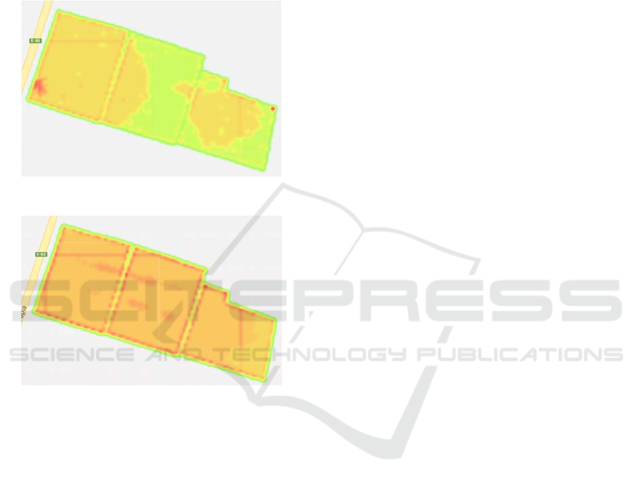
correspond to every vine in the orchard. Figures 1 and

2 show the NDVI observed in two of these dates as

an example of data representation.

Figure 1: NDVI observed on October 9

, 2014.

Figure 2: NDVI observed on December 3

, 2014.

It can be observed that when the red colour is

more intense, a greater value of the NDVI is

observed. On the other hand, when the green colour

is more intense, a lower value of the NDVI is

registered.

2.1 Proposed Method to Forecast the

NDVI

The method proposed for estimating the NDVI of the

orchard is summarized as follows:

 Step 1: The NDVI data of the first four dates (each

date is a variable of the algorithm) is used in order

to perform a clustering procedure. For this

clustering, the Fuzzy c-Means Clustering

Algorithm (FCM) proposed by Bezdek et al.

(1984) was applied. This algorithm requires the

number of clusters to be formed as a parameter.

For the case study, the algorithm was run 39

times, aiming to establish the clusters, which

varied in number from 2 to 40.

 Step 2: Once the clustering with different numbers

of clusters was obtained, the silhouette

representation of each cluster was used to evaluate

them. This function was developed by Rousseeuw

(1987). The number of clusters that achieves the

best value of the silhouette function was selected

and used for calculating the NDVI estimation.

This estimation is carried out in the following

step.

 Step 3: The NDVI estimation for the last date

(January 12

, 2015) was obtained by applying

neural networks. In this way, data from the first

four days was used to train the neural network

algorithm, while the last date was used to validate

the NDVI prediction.

In the following sub-sections, we explain in more

detail each step in our methodology.

It is important to notice that every step of the

methodology was executed using R software, version

3.4.3, in a Dell 321 PowerEdge R/730 server with

Intel Xeon E5 2623-v3 and 3 Ghz.

2.1.1 Step 1: Fuzzy c-Means Clustering

Algorithm (FCM)

The FCM was proposed by Bezdek et al., (1984) for

generating fuzzy partitions and prototypes for any set

of numerical data. The clustering criterion used to

aggregate subsets is a generalized least-squares

objective function. The FCM requires the choice of

one of three norms (Euclidean, Diagonal, or

Mahalonobis), an adjustable weighting factor that

controls sensitivity to noise and the number of

clusters needs to be defined. For the case study, we

used the Euclidean distance, a weighting factor value

of 1.1 and we varied the number of clusters from 2 to

40.

It is important to mention that the value of the

weighting factor requires a calibration in order to

improve the clustering results. As mentioned

previously, we used a weighting factor equal to 1.1.

The mathematical model developed for the FCM

algorithm is:

Min



,















(1)

Subject to











1, 1,…,,

(2)







0,1,…,,1,…,.2

(3)

ICORES 2019 - 8th International Conference on Operations Research and Enterprise Systems

190

Where:

n is the number of points,

k is the number of clusters,

is the degree of membership of a point i to a cluster

d(x

, c

) corresponds to the distance from a point i to

the centroid of a cluster j.

The centroid c

is calculated iteratively during the

algorithm execution, considering the values of u

. In

this way, when u

converges, that is, achieves less

variation than an epsilon, the FCM algorithm stops.

The result of this algorithm is the degree of

membership of each point i to each cluster j,

represented by u

For this case study, the distance d(x

, c

) was

calculated considering the Euclidean distance

between six coordinates. These six coordinates were

abscissa, ordinate, and the NDVI values of the first

four dates. In addition, for calculating the Euclidean

distance, it was necessary to normalize the abscissa

and ordinate. This normalization assigns to the

highest value a 1 and to the lowest value a 0.

2.1.2 Step 2: Application of Silhouettes

The silhouette function was proposed by Rousseeuw

(1987) and is based on the comparison of clusters’

tightness and separation. This silhouette shows which

objects lie well within their cluster and which ones

are merely somewhere in between clusters.

The evaluation of the 39 clusters obtained in Step

1 was carried out using the silhouette function in the

following way:

 Calculate the Euclidean distance from a given

point i of a cluster j to every point of the same

cluster A. Once all these distances are obtained,

calculate the average of these distances, which is

called average dissimilarity of i to all other objects

of A, a(i).

 Calculate the Euclidean distance from a given

point i of cluster A to each point of a given cluster

C (being C a different cluster from A). Then,

calculate the average of these distances. This

average is the average dissimilarity of i to all

objects of C, d(i, C).

 Once the averages d(i, C) for all C  A have been

computed, select the smallest of them and denote

it by b(i).

 With the values of a(i) and b(i), the function of

silhouettes s(i) must be calculated according to the

following equation:

 











max







,

(4)

The silhouette function s(i) varies from -1 to 1. When

s(i) is closer to 1 it means that a(i) < b(i) and we can

say that i is “well-clustered”. This is explained

because if s(i) is 1, it means that a(i) = 0, that is, all

points within the cluster A are very close, and also,

the maximum value between a(i) and b(i) will be b(i).

Therefore, the formula (4) will remain b(i)/b(i) = 1.

For more details of the silhouette interpretation, see

Rousseeuw (1987).

Using silhouettes, the clusters obtained in Step 1

were evaluated in order to select the one that had the

best s(i) value (closer to 1).

2.1.3 Step 3: Neural Network for NDVI

Forecast

A neural network algorithm was developed to

estimate the NDVI of each point i for January 12

2015, using the NDVI of the previous four dates

(October 9

, October 30

, November 11

and

December 3

of 2014). These four dates were divided

into a training sample (70% of data) and a validation

sample (30% of data); both samples were generated

randomly. Therefore, the observed NDVI on January

, 2015 was used to validate the obtained NDVI

forecast.

In the neural network algorithm, we used the

normalized data (values from 0 to 1) of the following

predictor variables: distance from a point i to the

centroid of each cluster j – d(x

, c

); the degree of

membership from point i to each cluster j (u

)

multiplied by its NDVI observed in the last date

where it was collected. For the case study, it

corresponds to the NDVI observed on December 3

In addition, the degree of membership u

and the

distance d(x

, c

) were computed in Step 1 and we had

3532 coordinates (points) for each date.

For training the neuronal network, 5, 7 and 10

neurons in only one hidden layer were tested. In this

way, the number of neurons that obtains the smallest

error, that is, the smallest mean absolute percentage

error (MAPE), is selected. For our case study, 7

neurons into one hidden layer obtained the smallest

MAPE, and then this number of neurons was selected.

The computational experimentation of the neural

network algorithm was done using the nnet package

of R. This package uses the logic or sigmoid function

as the activation function for the algorithm.

3 RESULTS

The main results obtained by the proposed method are

described in this section.

Using Data Mining Techniques to Forecast the Normalized Difference Vegetation Index (NDVI) in Table Grape

191

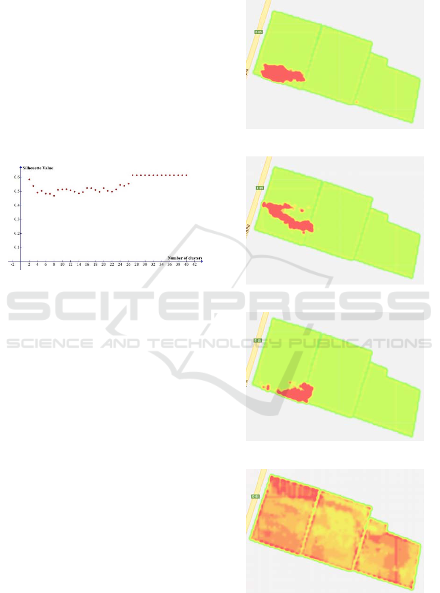
As mentioned previously, the FCM algorithm was

run 39 times for defining the clustering with different

numbers of clusters (from 2 to 40). After performing

this procedure, the silhouette function was applied for

evaluating every clustering. Figure 3 shows the

behaviour of the silhouette values calculated for each

clustering, which varies in number from 2 to 40. In

this figure, it is possible to observe that the silhouette

value converges to 0.6 from 27 clusters. Moreover,

this is the highest value of s(i). For this reason, the

selected number of clusters for executing the neural

network algorithm was 27. In Table A.1 of the

Appendix, the obtained silhouette values are

presented.

Figure 3: Silhouette values according to the number of

clusters.

An example of three clusters obtained by the FCM

algorithm are depicted in Figures 4, 5 and 6. The red

colour represents each cluster. These clusters belong

to the selected set of 27 clusters.

Once the best clustering according to the

silhouette function was selected, the neural network

algorithm was applied for estimating the NDVI of

each point in the orchard at time “t + 1”, that is, on

January 12

, 2015. In this algorithm, 54 predictor

variables were used, which were: 27 d(x

, c

) and 27

multiplied by its NDVI observed in the last date.

Figure 7 shows the observed NDVI on January 12

2015, while Figure 8 presents the estimated NDVI for

the same date by the neural network algorithm. In

these figures, similarly to Figures 1 and 2, when the

red colour is more intense, a greater value of the

NDVI is observed. On the other hand, when the green

colour is more intense, a lower value of the NDVI is

registered.

Figure 4: Cluster 1.

Figure 5: Cluster 2.

Figure 6: Cluster 3.

Figure 7: NDVI observed on January 12

, 2015.

ICORES 2019 - 8th International Conference on Operations Research and Enterprise Systems

192

Figure 8: Estimated NDVI for January 12

, 2015.

The NDVI forecast obtained by the neural

network algorithm presented a mean absolute

percentage error (MAPE) equal to 0.34% in the

validation sample and 1.83% in the test sample. It is

important to mention that a MAPE less or equal than

10% indicates that the accuracy (quality) of the

forecast is very good, according to the classification

proposed by Ghiani et al., (2004). In addition, we

obtained a very good NDVI prediction 40 days in

advance, being useful information for planning

agricultural activities such as harvesting.

4 CONCLUSIONS

The proposed method allowed predicting future

NDVI based on previous measurements with high

accuracy (MAPE of 1.83%).

In future researches, the following issues should

be explored:

 To forecast the quality and quantity of table

grapes in a given orchard according to the

predicted or measured NDVI. In this way, it

would be possible to plan harvesting.

 To model a harvesting plan according to the

grape’s quality and quantity forecast.

 To study the time frequency with which data must

be collected in order to analyse its impact on the

NDVI forecast.

 To analyse the possibility to reduce the number of

points to be sampled in a same cluster, since they

are homogeneous. In this way, it could be useful

to determine which points to sample, For

example, to study if the centroid of each cluster

could serve as a representative point

ACKNOWLEDGEMENTS

This work is supported by the Support Funding for

the Academic Development (FADA) of the

Departamento de Ingeniería Comercial of

Universidad Técnica Federico Santa María and by the

CYTED program through the thematic network

BigDSS-Agro, Project P515RT0123.

REFERENCES

Berger, A., Ettlin, G., Quincke, C., Rodríguez-Bocca, P.,

2018. Predicting the Normalized Difference Vegetation

Index (NDVI) by training a crop growth model with

historical data, Computers and Electronics in

Agriculture, article in press.

Bezde, J.C., Ehrlich, R., Full, W., 1984. FCM: The Fuzzy

c-Means Clustering Algorithm, Computers &

Geosciences, 10(2-3): 191-203.

Cunha, M., Marcal, A.R., Silva, L., 2010. Very early

prediction of wine yield based on satellite data from

VEGETATION, International Journal of Remote

Sensing, 31(12): 3125-3142.

Font, D., Tresanchez, M., Martínez, D., Moreno, J., Clotet,

E., Palacín, J., 2015. Vineyard yield estimation based

on the analysis of high resolution images obtained with

artificial illumination at night, Sensors, 15(4): 8284-

8301.

Fortes Gallego, R., Prieto Losada, M. D. H., García Martín,

A., Córdoba Pérez, A., Martínez, L., Campillo Torres,

C., 2015. Using NDVI and guided sampling to develop

yield prediction maps of processing tomato crop,

Spanish Journal of Agricultural Research, 13(1), e02-

004, 9 pages.

Ghiani, G., Laporte, G., Musmanno, R., 2004. Introduction

to logistics systems planning and control, John Wiley

& Sons Ltd, The Atrium, Southern Gate, Chichester,

West Sussex PO19 8SQ, England.

Ortega-Blu, R., Molina-Roco, M., 2016. Evaluation of

vegetation indices and apparent soil electrical

conductivity for site-specific vineyard management in

Chile, Precision Agriculture, 17(4): 434–450.

Pettorelli, N., 2013. The Normalized Difference Vegetation

Index, Oxford Scholarship, England.

Pôças, I., Paço, T.A., Paredes, P., Cunha, M., Pereira, L.S.,

2015. Estimation of Actual Crop Coefficients Using

Remotely Sensed Vegetation Indices and Soil Water

Balance Modelled Data, Remote Sensing, 7: 2373-2400.

Rousseeuw, P.J., 1987. Silhouettes: A Graphical Aid to the

Interpretation and Validation of Cluster Analysis,

Journal of Computational and Applied Mathematics,

20: 53-65.

Sun, L., Gao, F., Anderson, M. C., Kustas, W. P., Alsina,

M. M., Sanchez, L., Sams, B., McKee, L., Dulaney, W.,

White, W. A.,. Alfieri, J. G., Prueger, J. H., Melton, F.,

Post, K., 2017. Daily mapping of 30 m LAI and NDVI

Using Data Mining Techniques to Forecast the Normalized Difference Vegetation Index (NDVI) in Table Grape

193

for Grape Yield Prediction in California Vineyards,

Remote Sensing, 9(4): 317.

Yu, B., Shang, S., 2018. Multi-Year Mapping of Major

Crop Yields in an Irrigation District from High Spatial

and Temporal Resolution Vegetation Index, Sensors,

18(11): 3787.

APPENDIX

Table A.1: Silhouette values according to the number of

clusters.

# Clusters s(i) # Clusters s(i)

2 0.5829 22 0.4958

3 0.5363 23 0.5123

4 0.4902 24 0.5435

5 0.5027 25 0.5378

6 0.4817 26 0.5529

7 0.4812 27 0.6140

8 0.4672 28 0.6140

9 0.5104 29 0.6140

10 0.5120 30 0.6140

11 0.5138 31 0.6140

12 0.5062 32 0.6140

13 0.4965 33 0.6140

14 0.4836 34 0.6140

15 0.4935 35 0.6140

16 0.5225 36 0.6140

17 0.5213 37 0.6140

18 0.5088 38 0.6140

19 0.4947 39 0.6140

20 0.5210 40 0.6140

21 0.5023

ICORES 2019 - 8th International Conference on Operations Research and Enterprise Systems

194