
Exploring Medical Data Classification with Three-Way Decision Trees
Andrea Campagner
1,3
, Federico Cabitza
1,2
and Davide Ciucci
1
1
Dipartimento di Informatica, Sistemistica e Comunicazione,
University of Milano–Bicocca, viale Sarca 336 – 20126 Milano, Italy
2
IRCCS Istituto Ortopedico Galeazzi, via Galeazzi 4 – 20161 Milano, Italy
3
Datareg, Via Limonta, 89 – 20092 Cinisello Balsamo, Italy
Keywords:
Machine Learning, Uncertainty, Three–Way Decision, Medicine, Data Analysis.
Abstract:
Uncertainty is an intrinsic component of the clinical practice, which manifests itself in a variety of different
forms. Despite the growing popularity of Machine Learning–based Decision Support Systems (ML-DSS) in
the clinical domain, the effects of the uncertainty that is inherent in the medical data used to train and optimize
these systems remain largely under–considered in the Machine Learning community, as well as in the health
informatics one. A particularly common type of uncertainty arising in the clinical decision–making process
is related to the ambiguity resulting from either lack of decisive information (lack of evidence) or excess of
discordant information (lack of consensus). Both types of uncertainty create the opportunity for clinicians to
abstain from making a clear–cut classification of the phenomenon under observation and consideration. In
this work, we study a Machine Learning model endowed with the ability to directly work with both sources
of imperfect information mentioned above. In order to investigate the possible trade–off between accuracy
and uncertainty given by the possibility of abstention, we performed an evaluation of the considered model,
against a variety of standard Machine Learning algorithms, on a real–world clinical classification problem.
We report promising results in terms of commonly used performance metrics.
1 INTRODUCTION
In the recent years, Machine Learning (ML) has
gained the growing interest of the medical commu-
nity, for its promise to deliver more accurate Decision
Support Systems (DSS) (Deo, 2015; Obermeyer and
Emanuel, 2016; Kooi et al., 2017). These ML-based
DSSs (ML-DSSs), rather than being based on any ex-
plicit formalization of procedural knowledge, assist
the clinicians in their decisions on the basis of the hid-
den patterns that characterize large amount of medi-
cal data and that can be represented in terms of com-
plex statistical models (ML models) that are “learned”
through computational procedures.
In the medical community, it is widely acknowl-
edged (Fox, 2000; Rosenfeld, 2003; Simpkin and
Schwartzstein, 2016; Hatch, 2017) that uncertainty
is an intrinsic component of medical practice and
that several forms of uncertainty, like vagueness and
ambiguity (Parsons, 2001; Greenhalgh, 2013) affect
medical records and are mirrored in the medical data
that these contain.
This common condition of medical data, however,
has been largely ignored by ML researchers, despite
the fact that this uncertainty could undermine the va-
lidity of the data that are used to “train” the ML mod-
els above, thus affecting their performance and relia-
bility negatively (Cabitza et al., 2019a).
The authors of a recent review of the medical liter-
ature (Han et al., 2011) propose to distinguish among
three sources of potential uncertainty: this latter one
can arise from: the intrinsic indeterminacy of a phe-
nomenon (probability); the difficulty to comprehend
some aspects of the phenomenon (complexity); the
lack of reliability, credibility and adequacy of the in-
formation about the phenomenon (ambiguity).
In this paper we address two common types of this
latter form of uncertainty in medical decision mak-
ing: ambiguity due to lack of information; and am-
biguity due to lack of agreement in collaborative (or
multi-observer) settings. The first condition occurs
when a doctor deems the available evidence not ade-
quately accurate, reliable, or complete to take a rea-
sonable (i.e., not imprudent) decision and thus ab-
stains from it (Pauker and Kassirer, 1980; Lurie and
Sox, 1999). The second condition occurs when more
than one clinician are involved, they evaluate the pa-
tients’s condition collaboratively (and sometimes in-
dependently from each other, as in case of double
reading policies for diagnostic imaging, e.g. (Brown
Campagner, A., Cabitza, F. and Ciucci, D.
Exploring Medical Data Classification with Three-Way Decision Trees.
DOI: 10.5220/0007571001470158
In Proceedings of the 12th International Joint Conference on Biomedical Engineering Systems and Technologies (BIOSTEC 2019), pages 147-158
ISBN: 978-989-758-353-7
Copyright
c
2019 by SCITEPRESS – Science and Technology Publications, Lda. All rights reserved
147

et al., 1996)) and they cannot agree on a definitive in-
terpretation.
Both the conditions mentioned above are more
frequent than a lay person could imagine. In fact, the
uncertainty for lack of information is often the main
motivation for the so called ‘wait-and-see’ policy
(e.g., (Glynne-Jones and Hughes, 2012)), by which no
intervention is prescribed and the condition is moni-
tored over time to gain more decisive findings. In re-
cent times, the medical community has hosted a lively
debate about whether doctors should abstain from
prescribing exams and treatments more often than cur-
rently observed, with an emphasis on the mandate
not to harm (Grady and Redberg, 2010) and to avoid
over-diagnosis (Djulbegovic, 2004), that is classify-
ing as diseases (and treat) conditions that will never
evolve into serious illness. The second condition is
even more common, and denoted in the medical lit-
erature as either poor or moderate inter-rater agree-
ment (Gwet, 2014). For instance, discrepancy rates
for second interpretations of pediatric cases between
two health care facilities were found substantial with
disagreements that occurred in almost one case out
of two (Eakins et al., 2012). In real-world settings a
majority vote policy is usually adopted to take a deci-
sion and proceed despite the disagreements (Cabitza
et al., 2017). It is worthy of note that disagreements
are usually not due to errors (or minimally so), but
rather to the intrinsic ambiguity of the observed phe-
nomena (Cabitza et al., 2019a; Cabitza et al., 2019b).
The main consequence of these types of uncer-
tainty for the design of ML-DSS is that the gold-
standard target (or ground truth), which is fed as train-
ing data into ML algorithms, can no longer be con-
sidered a clear-cut classification. Consequently, the
assignment of a binary (or, more generally, multi-
class) label to each instance is no longer feasible, but
rather a three-valued (or more generally set-valued)
classification is needed, in which a set-valued labeling
{c
1
,...,c
k
} of a given instance means that the correct
classification is unknown, yet one among c
1
,...,c
k
.
Some authors have already tried to address ambi-
guity in computational terms: for instance, the work
of (Ferri and Hern
´
andez-Orallo, 2004) on Cautious
Classifiers, the work of (Yao, 2012) on Three–Way
Decisions, and the work of (Cour et al., 2011) on
learning from partial labels. These seminal works
notwithstanding, this aspect is seldom considered and
deployed in real–world applications. In fact, the stan-
dard approach to tackle uncertain decision problems
in the ML community consists in using probabilistic
methods, which in the considered setting regards the
assignment of a probability degree to each of the con-
sidered alternatives. However under this mainstream
approach, this soft probabilistic classification is usu-
ally converted into a clear-cut one, for example con-
sidering the assignment with the highest probability.
While this technique could be seen as an effective
way to control and eliminate uncertainty, it could also
be seen as discarding the intrinsically uncertain and
multi-faceted nature of the clinical phenomena (Cab-
itza et al., 2019a).
The goal of this work is to consider a ML model
with the capability to process ambiguity, and under-
take a comparative study with respect to a variety
of traditional ML algorithms applied to a real-world
clinical decision problem. Specifically, we will eval-
uate the considered model under the problem of as-
sessing either the improvement or the worsening of
mental health after a surgical operation, as this con-
struct is measured by the mental score that can be
computed on the basis of the responses that patients
give when responding to the Short Form 12 (SF12)
survey, a standard and widely-used questionnaire for
routine monitoring and assessment of care outcomes
in adult patients (Ware et al., 1996; Ware et al., 1998).
We will consider two different classification tasks:
1. The first case is analogous to cautious classifica-
tion and three–way classification: in this case, the
target classification is binary, but the classifier,
when not sufficiently certain on the classification
to assign, is able to predict a three-way output.
This latter category is not yet a further class, but
rather a tertium (cf. Aristotle), a Mu value (cf.
Zhaozhou) or, more prosaically, an explicit user
missing that is intended to emulate the abstention
behaviour mentioned above.
2. The second case is a generalization of both cau-
tious classification and learning from partial la-
bels (Cour et al., 2011): for this reason we call
it three–way in/three–way out classification. In
this original approach, both the input (that is the
training data) and the output (that is the predicted
target variable) can present abstention decisions
explicitly; given that the training input is three–
way, in its predictions the ML algorithm can ei-
ther dispel the uncertainty by yielding a precise
classification, if it is “certain” of this decision; or,
otherwise, the algorithm can resort to abstention,
and propagate the uncertainty onto the predicted
output.
It should be noted that both the tasks described above
are essentially different from both multi–class and
multi–label classification (see Figure 1 for a graphi-
cal representation of the differences):
• Multi–class classification assumes a certain input
and the goal is to predict a certain output which
HEALTHINF 2019 - 12th International Conference on Health Informatics
148
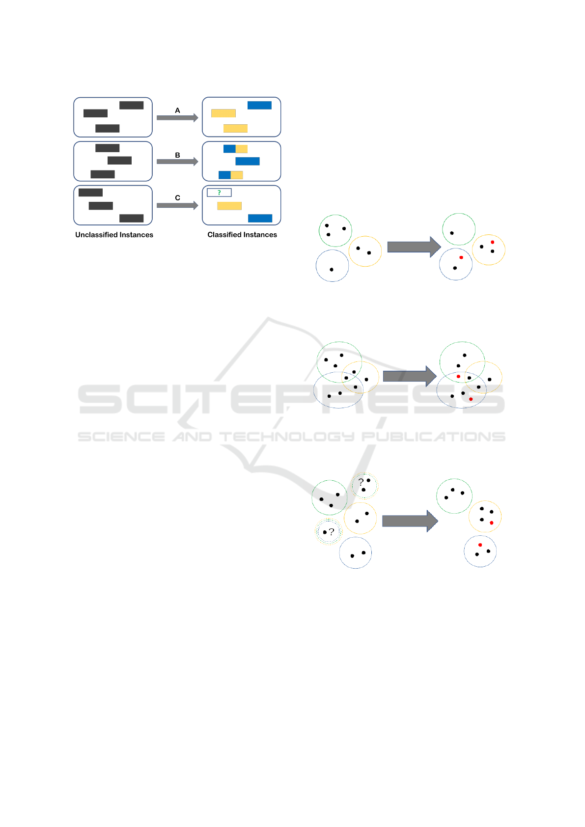
Figure 1: A representation of multi–class (A), multi–label
(B) and three–way classification (C).
can assume more than two values (only one for a
single instance);
• Multi–label classification (Tsoumakas and
Katakis, 2007) assumes a set–valued, yet certain,
input and the goal is to predict a certain set–
valued output. In this latter case the classes are
assumed to be non–exclusive;
On the other hand, as explained previously, cau-
tious classification assumes a binary (more in general
multi–class) input, but the goal is to predict an uncer-
tain set–valued output which should contain the real
label with high confidence. Finally, in the three–way
in/three–way out approach that we propose, the input
itself is assumed to be set–valued and uncertain and
the goal is to produce an uncertain set–valued output
(which, possibly, is less uncertain than, but consistent
with, the input).
The rest of this work is organized as follows: in
Section 2, we will provide an introduction to the novel
ML model. We will then describe the dataset that we
used for its evaluation, as well as the model evalua-
tion setting that we employed; in Section 3, we will
describe in detail the results obtained from the model
evaluation experiment described in Section 2; finally,
in Section 4, we will discuss the obtained results, also
in the light of further improvements and future works.
2 METHODOLOGY
As mentioned in Section 1, the goal of this work is
the study and evaluation of ML models with the abil-
ity to deal with a specific form of lack of knowledge,
resulting from the presence of abstention decisions.
More specifically we will consider two different set-
tings: in the first one (which can be seen as an in-
stance of cautious classification) the input labeling is
binary, but the model is given the ability to abstain on
the instances it deems as unclear or uncertain, with the
purpose of avoiding classification errors; in the sec-
ond one, which we call three–way in/three–way out
classification, both the input and output labelings are
allowed to contain uncertain instances which are asso-
ciated with an abstention decision. A graphical illus-
tration of the differences among the various ML set-
tings (multi–class, multi–label, learning from partial
labels and cautious classification) is shown in Figures
2, 3, 4, 5.
Figure 2: An example of multi–class classification: each
object (represented as a dot) is associated with only one
class (represented as a colored circle). Red dots represent
misclassified objects.
Figure 3: An example of multi–label classification: in this
setting the classes (represented as colored circles) are not
exclusive, thus objects (represented as dots) can be associ-
ated with multiple classes (objects in the intersections). Red
dots represent misclassified objects.
Figure 4: An example of learning from partial labels (three–
way input): in this setting the classes (represented as col-
ored circles) are exclusive, but the assignment of objects
(represented as dots) in the input could be uncertain (repre-
sented as multi–colored dashed circles). The output of the
classifier assigns a single class to each object in a consistent
way. Red dots represent misclassified objects.
In particular, in order to tackle the described clas-
sification settings, we will consider a model, intro-
duced in (Campagner and Ciucci, 2018), which is a
generalization of Decision Tree Learning based on
Three–Way Decisions and Orthopairs (Ciucci, 2011;
Exploring Medical Data Classification with Three-Way Decision Trees
149

Figure 5: An example of cautious classification (three–way
output): each object (represented as a dot) is associated with
only one class (represented as a colored circle). The classi-
fier has the ability to abstain on objects it deems uncertain
(in order to avoid misclassifications).
Ciucci, 2016). The rest of this section proceeds as fol-
lows: in Section 2.1.1 we will provide a concise intro-
duction to the necessary mathematical backgrounds;
then, in Section 2.1.2 we will introduce the consid-
ered ML model; finally, in Section 2.2 we will detail
the considered classification problem and the model
evaluation setting employed.
2.1 Three–Way Decision Tree Learning
2.1.1 Introduction to Orthopartitions
We define an orthopair on a given set U as a pair of
disjoint sets hP,Ni (i.e., such that P ∩ N =
/
0). From
these two sets we can also define the boundary or un-
certain region as U nc = (P ∪ N)
c
. In a classification
context, we can understand P as the set of certainly
positive examples, N as the set of certainly negative
examples and Unc as the set of uncertain examples.
Thus, in the terminology of (Ferri and Hern
´
andez-
Orallo, 2004), the output of a Cautious Classifier can
be seen as an orthopair where the abstention decision
⊥ corresponds to examples in Unc. We say that a set
S is consistent with an orthopair O if it holds that
x ∈ P ⇒ x ∈ S and x ∈ N ⇒ x /∈ S. (1)
We say that two orthopairs O
1
= hP
1
,N
1
i,O
2
=
hP
1
,N
1
i are dis joint if the following conditions hold:
P
1
∩ P
2
=
/
0; (2a)
P
1
∩Unc
2
=
/
0 and Unc
1
∩ P
2
=
/
0. (2b)
More generally, considering a multi-class classi-
fication setting, we can define the concept of an or-
thopartition, understood as a generalization of clas-
sical partitions, as a multi–set of orthopairs O =
{O
1
,...,O
n
} satisfying:
∀O
i
,O
j
∈ O O
i
,O
j
are disjoint; (3a)
\
i
N
i
=
/
0; (3b)
∀x ∈ U(∃O
i
s.t. x ∈ Unc
i
)
⇒ (∃O
j
with i 6= j s.t. x ∈ U nc
j
). (3c)
Thus, as implied by the axioms, an element in
(more than one) boundary is an element whose class
assignment is uncertain.
We say that a partition π is consistent with an or-
thopartition O iff ∀O
i
∈ O, ∃S
i
∈ π such that S is con-
sistent with O
i
and the S
i
s are all disjoint. We denote
as Π
O
= {π|π is consistent with O} the set of all par-
titions consistent with O.
The logical entropy (Ellerman, 2013) (also known
as Gini impurity index (Breiman et al., 1984)) of a
partition π is defined as:
h(π) =
|dit(π)|
|U|
2
(4)
where dit(π) is defined as:
dit(π) = {(u,u
0
) ∈ U ×U|u ∈ π
i
,u
0
∈ π
j
,i 6= j} (5)
Given the set of compatible partitions we can provide
a generalized definition of logical entropy
ˆ
h, which is
used in learning Three–Way Decision Trees:
h
∗
= min{h(π)|π ∈ Π
O
} (6a)
h
∗
= max{h(π)|π ∈ Π
O
} (6b)
ˆ
h =
h
∗
(O) + h
∗
(O)
2
(6c)
2.1.2 Introduction to Three–Way Decision Tree
Learning
Decision Trees are a popular decision–making model,
mainly due to their interpretability and their similar-
ity to the human decision–making process, also in the
clinical setting (Podgorelec et al., 2002; Dowding and
Thompson, 2004; Dowie, 1996). Basically, they can
be described as trees in which each internal node rep-
resents a test on a given independent variable and each
leaf corresponds to a decision. Thus, in the classi-
fication setting that we are considering, each leaf is
the decision associated with the independent variables
values in the respective path from the root, an exam-
ple is shown in Figure 6. Given their popularity in
the decision-making and ML community, a variety of
Vision Loss
Pain
Uveitis
Cataract
Pain
Optic Neuritis
Retinal detachment
slow
yes
no
rapid
yes
no
Figure 6: An example Decision Tree, showing a limited ex-
ample of optic disease diagnosis.
HEALTHINF 2019 - 12th International Conference on Health Informatics
150

Decision Tree Learning algorithms have been devel-
oped; among them, we recall C4.5 (Quinlan, 1993)
and CART (Breiman et al., 1984), which are based on
the outline given in Algorithm 1.
Algorithm 1: Decision Tree Induction Algorithm.
Input: Dataset D
Output: Decision Tree built on D
1 for feature a, split value v
a
do
2 Compute entropy h
a,v
a
with respect to D
3 end
4 if stopping criterion reached then
5 Choose optimal classification
6 else
7 Select feature a
∗
, split value v
∗
a
with minimal
entropy and create a decision node;
8 Recur on the subsets of D determined by the
values of a
∗
,v
∗
a
;
9 end
In (Campagner and Ciucci, 2018), the authors
proposed a generalized Three–Way Decision Tree
(TWDT) Learning model, based on Three–Way Deci-
sions and orthopartitions, with the ability to both ex-
press abstention decisions and induce Decision Trees
in a semi–supervised manner. This algorithm gen-
eralizes the classical ones on two aspects: the com-
putation of the entropy h with respect to the dataset
D, and the procedure to select the optimal classifica-
tion. In the following explanation, for simplicity but
without loss of generality, we will consider only cate-
gorical features (i.e., nominal features with a discrete
unordered set of possible values).
Semi–Supervised Entropy Computation.
The classification, in this setting, could be
missing for some of the instances, that is
∀x ∈ D, C(x) ∈ {P,N,⊥} where ⊥ represents a
missing classification. Such a dataset naturally
describes an orthopartition and we can then simply
modify the entropy calculation by considering the
value of
ˆ
h. This computation easily generalizes
to the multi–class case (this setting, which is a
generalization of multi–class learning, is known as
Learning from Partial Labels (Cour et al., 2011)):
if Cl is the set of possible clear-cut classifications,
then, ∀x ∈ D, C(x) ∈ 2
Cl
, which, again, naturally
describes an orthopartition.
Selection of the Optimal Classification. Let D =
{x
1
,...,x
|D|
} ⊆ X be a given dataset with a set of fea-
tures {a
1
,...,a
m
} and a single target classification fea-
ture C. We will consider, for simplicity, only the bi-
nary classification approach, that is ∀x ∈ D, C(x) ∈
{P,N}, while the classifier would also have the op-
tion of abstaining (i.e., the output of model M over in-
stance x is allowed to be M(x) ∈ {P, N,Unc} where, as
previously specified, x ∈ Unc means that model M ab-
stains in assigning a classification to x). Let τ ∈ (0,1)
be a probability threshold, which represents the prob-
ability level under which the classifier will make an
abstention decision. Let D
a
i
= {x ∈ D|v
a
(x) = v
a
i
} be
the set of instances that have value v
a
i
for feature a.
We associate to D
a
i
the optimal classification :
C
a
i
= argmax
j∈{P,N}
{
|{x ∈ D
a
i
|C(x) = j}|
|D
a
i
|
} (7)
Then, if
P(C
a
i
) =
|{x ∈ C
a
i
}|
|D
a
i
|
≥ τ (8)
the algorithm would select C
a
i
as the optimal classi-
fication, otherwise the abstention decision ⊥ would
be selected. If the target classification is allowed to
be expressed in terms of three–way decisions (i.e.,
∀x ∈ D,C(x) ∈ {P,N,Unc}) then the probability of the
optimal classification should be changed as follows:
P(C
a
i
) =
1
2
∗
|{x ∈ D
a
i
|C(x) = ⊥}|
|D
a
i
|
+
|{x ∈ C
a
i
}|
|D
a
i
|
. (9)
For a more general and flexible formulation based on
decision costs and applicable to the multi–class and
learning from partial labels approaches we refer to
the original article (Campagner and Ciucci, 2018).
2.2 Model Evaluation Setting
2.2.1 Description of the Dataset
As already introduced in Section 1, the evaluation of
the model will regard the prediction of improvement
or worsening of mental health, as measured by the
mental score of the SF12 survey. More specifically,
the real–world considered dataset has been extracted
from an electronic specialty registry, called Datareg,
which is adopted to record joint replacement cases
at the Orthopedic Institute Galeazzi of Milan (Italy).
This dataset consists of 462 instances characterized
by the following 10 attributes (9 predictor features,
and 1 target variable):
• Age at hospitalization, numeric;
• Sex, categorical (Male or Female);
• Pre-Operative Visual Analog Scale (VAS) Pain
score (McCormack et al., 1988), numeric;
Exploring Medical Data Classification with Three-Way Decision Trees
151

• Pre-Operative Body–Mass Index (BMI) (Khosla
and Lowe, 1967), numeric;
• Knee Society Score (KSS) Pain (KSS-P), KSS
Function (KSS-F) and KSS Stability (KSS-S) Pre-
Operative scores (N. Insall et al., 1989), numeric;
• Pre-Operative SF12 Mental Score (SF12-MS),
numeric;
• Pre-Operative SF12 Physical Score (SF12-PS),
numeric;
• Delta SF12 Mental Score (DSF12-MS), defined as
the difference between the SF12-MS 6 months af-
ter the operation and the pre-operative SF12-MS;
numeric. This is our target variable.
We then performed a pipeline of pre–processing op-
erations:
1. Binarization of the Sex variable, in order to con-
vert all variables in numeric form;
2. Imputation of the missing values (for the variables
VAS, BMI, KSS-P, KSS-F and KSS-S), by using
a simple median imputation strategy;
3. Normalization of all the (originally) numeric pre-
dictor features.
We then proceeded to create two different datasets,
one for each of the considered classification tasks:
1. For the creation of the first dataset we simply bi-
narized the target variable, mapping values < 0 to
the label 0 and values ≥ 0 to the label 1;
2. For the creation of the dataset with abstention de-
cisions, we divided the universe in three by map-
ping values < −6.24 to label 0, values −6.24 ≤
x ≤ 6.24 to label ⊥ and values > 6.24 to label 1 (as
suggested in (Utah Department of Health, 2001)).
In this step, the above arbitrary threshold can be
asymmetric, according to domain expertise or em-
pirical studies, or be based on the observed error
variance or other similar indicators, like the mini-
mal detectable change and the minimal clinically
important difference, associated with the consid-
ered scores, e.g., (Impellizzeri et al., 2011).
The resulting datasets were both strongly unbalanced:
in the first dataset there were 382 instances with label
1 and 80 instances with label 0; in the second dataset
there were 310 instances with label 1, 37 instances
with label 0 and 115 instances with label ⊥. For this
reason, we performed a class reweighting (McCarthy
et al., 2005) procedure in order to place, during the
training phase of the algorithms, more emphasis to
instances in minority class.
2.2.2 Model Comparison Setting
After the construction of the two training datasets, we
designed an experiment in order to compare the con-
sidered model with a selection of classical ML algo-
rithms. Given the relatively small size of the sample
we did not perform an initial split of the dataset into
training and testing datasets; instead, we performed a
k–fold cross–validation, with k = 6, when estimating
the accuracy scores and performing hyper–parameter
selection of the considered models. More specifically,
given the imbalanced nature of the datasets we com-
pared the models on the basis of three criteria:
• Balanced Accuracy (BalAcc) (Mower, 2005), de-
fined as
True Positive Rate + True Negative Rate
2
(10)
allowing us to compare models more accurately
by considering, separately, accuracy on instances
labeled as 1 and as 0;
• Accuracy (Acc), defined simply as
True Positives + True Negatives
N
(11)
.
In order to evaluate the considered three–way deci-
sion tree model, for which the output classification
could be one of {1,0,⊥}, we redefined the above
measure in a way reminiscent of One vs Rest multi–
class classification (Bishop, 2006). Specifically, we
compute two values of balanced accuracy: the first
value BalAcc
0
is computed by aggregating 0 and ⊥ la-
bels, the second value BalAcc
1
is similarly computed
by aggregating 1 and ⊥ label. The value of the bal-
anced accuracy is then computed as their average:
ˆ
BalAcc =
BalAcc
0
+ BalAcc
1
2
(12)
We redefined the accuracy measure similarly. For
evaluation of the Three–Way Decision Tree, as sug-
gested in (Ferri and Hern
´
andez-Orallo, 2004), we also
computed the values of the considered metrics with-
out taking in consideration the predicted abstentions:
these values were used, in particular, for the compu-
tation of the ROC curves as detailed in Section 2.2.2
and for evaluating if the algorithm could outperform
other models when considering only the predictions
on which it was sufficiently “confident”. In this case,
we also computed the value of another metric that we
called Abstention Rate (AR), defined simply as:
AR =
Abstentions
N
(13)
Given the differences among the two consid-
ered decision problems, we also made some dataset–
specific decisions as follows.
HEALTHINF 2019 - 12th International Conference on Health Informatics
152

Binary Input, Three–Way Output. In regard to
this dataset, which corresponds to a cautious classifica
ion problem,we compared the Three–Way Decision
Tree algorithm described in Section 2.1.2 with the
following algorithms: K–Nearest Neighbors (KNN)
(Altman, 1992), Logistic Regression (McCullach and
Nelder, 1987), Linear Discriminant Analysis (LDA)
(Fisher, 1936), Na
¨
ıve Bayes (Russell and Norvig,
2009) with Gaussian variables, Support Vector Ma-
chines (SVM) (Boser et al., 1992) with Radial Ba-
sis Function kernels, Multilayer Perceptron (MLP)
(Goodfellow et al., 2016) with Rectified Linear Units
(ReLU) (Glorot et al., 2011) and Gradient Boosting
(Friedman, 2001). To compare the ML algorithms,
we also computed for each model the Receiver Op-
erating Characteristic (ROC) curves (Fawcett, 2006),
in order to analyze the performance of the algorithms
at varying operating points by plotting different val-
ues of True Positive Rate (TPR) at varying levels of
False Positive Rate (FPR):
T PR =
True Positives
True Positives + False Negatives
(14a)
FPR =
False Positives
False Positives + True Negatives
(14b)
To better analyze the performances of the Three–Way
Decision Tree model we also considered the variation
of classification accuracy with respect to the varying
abstention costs (Ferri and Hern
´
andez-Orallo, 2004).
Three–Way Input, Three–Way Output. In this
context, which corresponds to three–way in/three–
way out classification that we introduced previously,
we evaluated the Three–Way Decision Tree model
against the Label Propagation algorithm (Zhu and
Ghahramani, 2002). Given the complexity of per-
forming ROC analysis in this context, we simply eval-
uated the algorithms on the basis of the two previously
defined measures and respective confusion matrices.
Furthermore, we considered the variation of classifi-
cation accuracy with respect to the varying abstention
costs.
3 RESULTS
In this section we will describe the results obtained
via the model evaluation experiment detailed in Sec-
tion 2, specifically: in Section 3.1 we will present the
results for the dataset with binary input and three–way
output, and in Section 3.2, we will present the results
for the dataset with three-way input and output.
3.1 Results for the Binary Input,
Three–Way Output Dataset
The measured balanced accuracy and accuracy
values, along with the selected optimal hyper–
parameters, for the algorithms listed in Section 2.2.2
are summarized in Table 1.
As can be easily observed, the Three–Way De-
cision Tree algorithm performed best under the Bal-
Acc metric, with the Na
¨
ıve Bayes performing simi-
larly, and both obtaining relatively high values of ac-
curacy measures, while the value of balanced accu-
racy < 0.75 could easily be explained with the dif-
ficulty of predicting the minority class (in fact for
both algorithms we registered a True Negative Rate of
around 0.55). It can also be observed that, as expected
given the imbalanced nature of the dataset, the accu-
racy measure, when taken alone, was not sufficiently
informative. For instance, the LDA, KNN, MLP and
Gradient Boosting algorithms performed significantly
worse with respect to balanced accuracy, but compa-
rably or better than other algorithms with respect to
accuracy. This could be explained by the fact that
these classifiers produced highly skewed predictions,
greatly favoring the majority class.
Figure 7: Variation of balanced accuracy with respect to the
τ parameter.
When considering the performance of the Three–
Way Decision Tree without taking in consideration
the abstention decisions, it could be seen that the algo-
rithm significantly outperforms the other considered
approaches. As can be seen in the Confusion matrix,
shown in Table 2, even with τ = 0.7 the algorithm
classifies with high confidence more than half of the
dataset, achieving (considering the class imbalance) a
high accuracy for the minority class. It is also to note
that the accuracy for the TWDT without taking the
abstentions in consideration is lower than the one for
TWDT with τ = 0.2: this effect is due to the fact that
the τ = 0.2 TWDT produced a prediction favoring the
Exploring Medical Data Classification with Three-Way Decision Trees
153
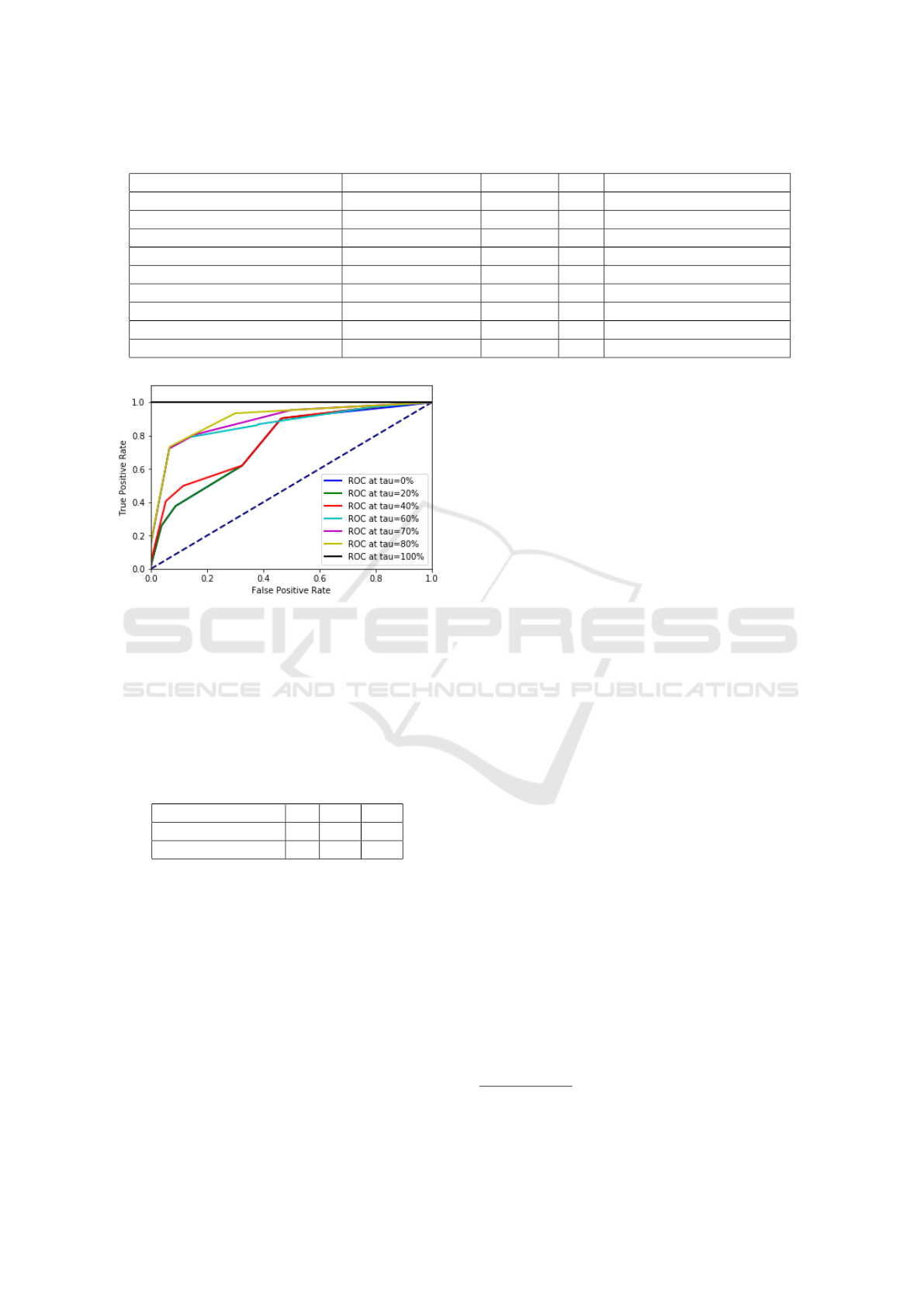
Table 1: Metrics results and selected hyper–parameters for the Binary Input, Three–Way Output Dataset.
Algorithm Balanced Accuracy Accuracy AR Hyper–Parameters
TWDT 0.72 0.84 0.0 Depth = 2, τ = 0.2
TWDT (Only predicted values) 0.82 0.81 0.50 Depth = 2, τ = 0.7
KNN 0.62 0.82 - k = 5
Logistic Regression 0.70 0.73 - -
LDA 0.64 0.83 - -
Na
¨
ıve Bayes 0.72 0.82 - -
SVM 0.70 0.74 - -
MLP 0.67 0.85 - Layers = 5, Nodes = 100
Gradient Boosting 0.65 0.85 - Estimators = 30, Depth = 2
Figure 8: Variation of the ROC curves with respect to the τ
parameter.
majority class, which obviously boosts the accuracy,
while the τ = 0.7 TWDT, as shown in Table 2, pro-
duced a more balanced prediction (thus favoring an
high value of balanced accuracy).
Table 2: Confusion matrix for the optimal hyper-parameters
of the TWDT algorithm, without considering the abstention
decisions.
Actual \ Predicted 0 1 ⊥
0 43 7 30
1 38 144 200
In order to provide a more fine-grained compari-
son of the considered algorithms, we also performed a
ROC analysis, comparing the respective ROC curves:
the resulting curves can be seen in Figure 9.
As can be easily seen, the ROC curve of the
TWDT algorithm (for which, as explained in Section
2.2.1, we considered only the predicted values, with
the hyper–parameters illustrated in Table 1) encloses
all the other curves, being the one curve more sim-
ilar to the optimal curve (i.e., the curve touching the
left and top borders). This provides a more significant
measure of the fact that the added flexibility, given by
the possibility of abstaining from decision, allows the
TWDT model to out–perform the other algorithms by
focusing only on the predictions for which it is suf-
ficiently confident: that is, the possibility of absten-
tion offers an interesting trade–off where one can in-
crease the accuracy (and confidence) of the prediction
by simply allowing the algorithm to abstain on some
instances. In order to more systemically study this
trade–off effect, we also considered the variation of
the balanced accuracy and the ROC curves with re-
spect to the variation of the τ parameter, for which the
results are shown in Figure 7 and Figure 8.
As expected, and illustrated in (Ferri and
Hern
´
andez-Orallo, 2004), with increasing levels of τ
the algorithm produces more precise predictions, by
simply discarding all the observations for which its
predictions would not be sufficiently confident. This
trade–off effect is best explained by looking at Figure
8 which clearly shows how increasing τ also increases
the accuracy of the algorithm but decreases its cover-
age
1
(illustrated by the gap among the curves). Note
also that the ROC curves, although depicted as con-
tinuous curves in Figure 8, can actually have discon-
tinuities due to operating points for which no actual
instance is classified, i.e., when the probability score
of all predictions is lower than τ.
3.2 Results for the Three–Way Input,
Three–Way Output Dataset
The measured balanced accuracy and accuracy
values, along with the selected optimal hyper–
parameters, for the algorithms listed in Section 2.2.2
are synthesized in Table 5.
As it can be easily seen, in this context the TWDT
algorithm, when considering the value of
ˆ
BalAcc and
ˆ
Acc, performs worse than the Label Propagation algo-
rithm, albeit they differ significantly only for the value
of the accuracy. In regard to the TWDT algorithm not
considering the abstention decision, the results im-
prove for both the metrics (as expected) with only a
1
By coverage we intend the proportion of instances that
are classified with respect to the abstentions.
HEALTHINF 2019 - 12th International Conference on Health Informatics
154
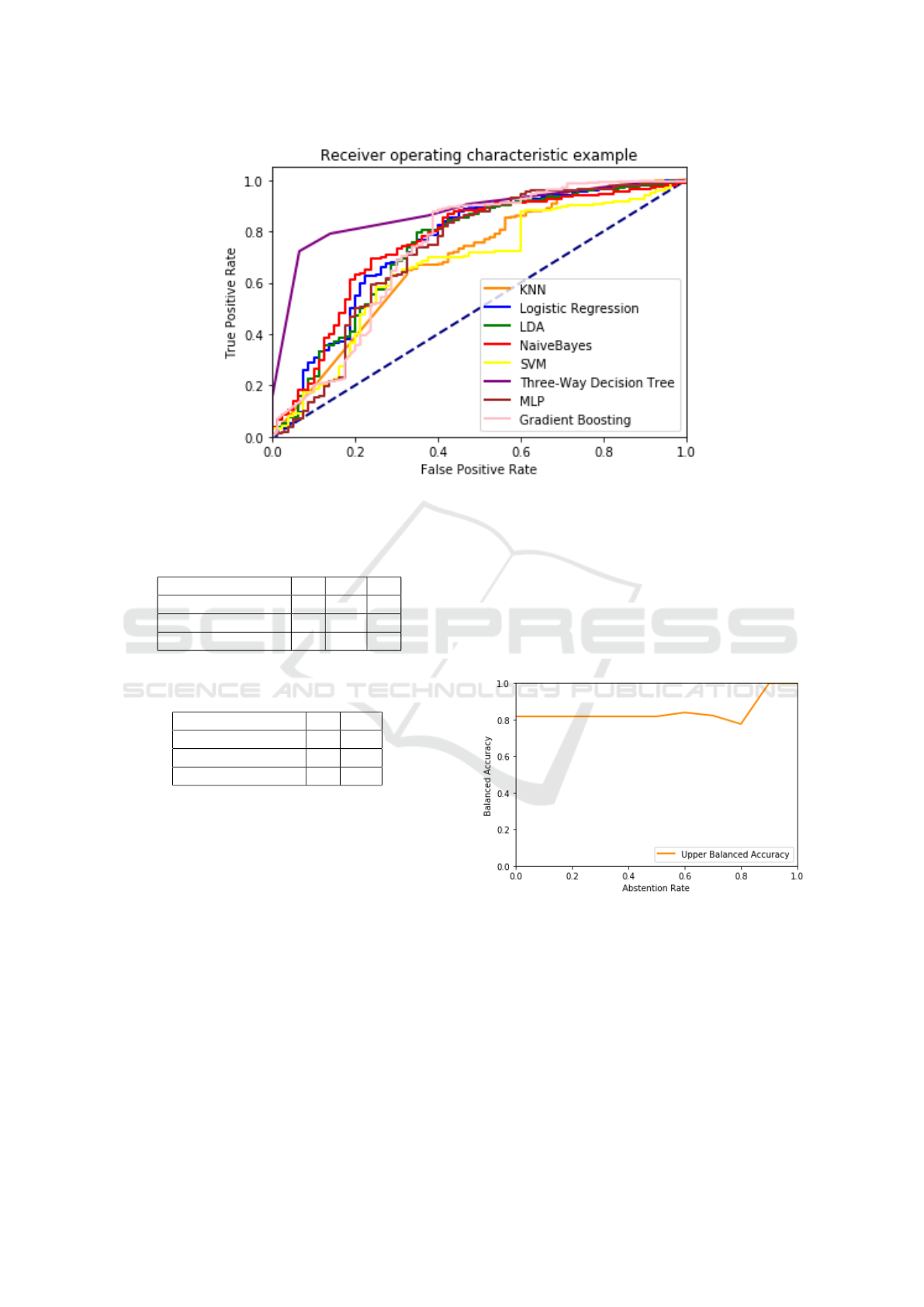
Figure 9: Comparison of ROC curves for the considered algorithms.
Table 3: Confusion matrix for the optimal hyper-parameters
of the TWDT algorithm, without considering the abstention
decisions.
Actual \ Predicted 0 1 ⊥
0 13 18 6
1 57 212 41
⊥ 41 61 13
Table 4: Confusion matrix for the optimal hyper-parameters
of the Label Propagation algorithm.
Actual \ Predicted 0 1
0 9 28
1 1 309
⊥ 13 102
moderate increase in the AR. However, while the al-
gorithm outperforms Label Propagation with respect
to the balanced accuracy, it still performs worse with
respect to the accuracy. As can be seen in the Confu-
sion Matrices, shown in Table 3 and Table 4, the high
accuracy obtained by the Label Spreading algorithm
could be explained by observing that the algorithm
produces a highly skewed prediction placing most of
the instances in the majority class. Conversely the
TWDT algorithm makes a much less skewed predic-
tion, with a balance among the predicted classes more
similar to the one given by the algorithms described in
Section 3.1 (i.e. it achieves high performance with re-
spect to the majority class, and little higher than ran-
dom performance on the minority class) and its errors
are thus much more probably due to the class imbal-
ance (in this case even more extreme than that of Sec-
tion 3.1). Thus, we can conclude that the result given
by the TWDT algorithm is more representative of the
real performance of the algorithm on this dataset, as
shown by the fact that it exhibits a higher value of
balanced accuracy. Also in this case, in order to study
the abstention–accuracy trade–off, we considered the
variation of the balanced accuracy with respect to the
variation of the τ parameter, for which the results are
shown in Figure 10.
Figure 10: Variation of balanced accuracy with respect to
the τ parameter.
4 CONCLUSION
In this work we studied the impact of a specific type
of uncertainty, the classification ambiguity that com-
monly arises in clinical decision making, on ML algo-
rithms; that is how the lack of knowledge that derives
from refraining from making a clear–cut decision, in
its turn due to a lack of adequate and sufficient evi-
Exploring Medical Data Classification with Three-Way Decision Trees
155

Table 5: Metrics results and selected hyper–parameters for the Three–Way Input Input, Three–Way Output Dataset.
Algorithm Balanced Accuracy Accuracy AR Hyper–Parameters
TWDT 0.76 0.74 0.0 Depth = 20, τ = 0.2
TWDT (Only predicted values) 0.84 0.79 0.13 Depth = 20, τ = 0.6
Label Propagation 0.78 0.87 - γ = 190
dence or of agreement on the available one, far from
being obliterated by unrealistic data-quality driven
policies, rather can be leveraged to design novel com-
putational aids capable of yielding either more accu-
rate or more informative advice, that is more adequate
tools for medical co-agencies (Thraen et al., 2012)
than the current ones (Castaneda et al., 2015).
In particular, we proposed a specific ML al-
gorithm that can directly manage this type of un-
certainty, and compared it with traditional ML ap-
proaches. In doing so, we could understand if this
added flexibility could result in better and more reli-
able predictions. Specifically, we evaluated the con-
sidered model, which represents an extension of the
popular Decision Tree Learning approach based on
Three–Way Decision Theory, on a real–world predic-
tion problem, namely the prediction of post-operative
improvement in mental health as represented by the
SF12 Mental score, considering two different ap-
proaches: cautious classification, and our novel ap-
proach, three–way in/three–way out classification. In
both cases, the considered algorithm outperformed
the other evaluated algorithms with respect to the
most suitable performance measure (i.e., balanced ac-
curacy) given the highly unbalanced nature of the
datasets. The obtained results clearly show that the in-
creased flexibility given by the possibility of express-
ing an abstention decision is able to increase the per-
formance and the significance of the predictions by
allowing the algorithm to provide a prediction only
for the instances for which the achieved confidence is
sufficient.
The three-way in/three-way out approach that we
propose has some implications on how medical data
are produced and recorded. In regard to the input of
ML algorithms, doctors could be finally allowed to
record richer and truer data out of their interpretations
of complex phenomena, with no need to hide their
perplexities and uncertainties under the rug of clear-
cut classifications that simply do not apply to their pa-
tients’ conditions. Despite the common tendency of
medical practitioners to accept and cope with vague
situations on a daily basis, current Electronic Medi-
cal Records are designed to obliterate this dimension,
forcing the adoption of disjoint categories, and man-
dating the imputation of values in the name of the ide-
als of completeness and precision, while not requir-
ing, for instance, to record the degree of confidence
with which a diagnosis is given along with the diag-
nostic or prognostic indication itself. On the other
hand, in regard to the output of ML algorithms, our
method can provide doctors with indications that, al-
though seemingly more affected by uncertainty, nev-
ertheless can be more informative and closer to their
mental models, which deal with uncertainty in richer
and more creative ways than computer and data sci-
entists usually are used to (Berg, 1997). This kind
of uncertainty-aware decision aids could also act as
training tools, which contribute in addressing what
has been called “the greatest deficiency of medical ed-
ucation throughout the twentieth century”, that is fail-
ing to train doctors about clinical uncertainty (Djulbe-
govic, 2004). Moreover in our view, providing algo-
rithms with the capability of working with abstention
decisions (either in the input, by the physicians, or in
the output, by the predictive algorithm) could in prin-
ciple foster the iterative interaction between the ML–
based DSS and the clinician (Holzinger, 2016), so that
this latter one can progressively refine the predictions
in a process that could be seen as a generalization of
the Active Learning setting (Settles, 2012).
In light of the promising results obtained, we plan
to expand this study by considering the following fu-
ture works:
• Firstly, we plan to expand this study by consid-
ering a wider variety of datasets, in order to bet-
ter analyze the performance increase given by the
possibility of abstention and establish its statisti-
cal significance;
• While Decision Trees offer several advantages, in
terms of simplicity and interpretability of the in-
duced models, they still represent a limited model
from an expressivity point of view (e.g., in re-
gard to smooth functions). We plan to consider
if endowing more sophisticated algorithms (such
as Random Forest, SVMs or Deep Learning algo-
rithms (Goodfellow et al., 2016)) with the same
ability of working with abstention decisions could
result in even better performance increases;
• We plan to apply the three–way in/three–way out
approach to multi–observer settings where con-
sensus cannot be achieved by either simple or
statistically significant majority (Svensson et al.,
2015);
• Consequently, we plan to consider three-way pre-
HEALTHINF 2019 - 12th International Conference on Health Informatics
156

dictor features, that is to allow abstentions not
only in the target variable of both the input (i.e.,
training) and the output (i.e., predicted) data, but
also in regard to any other feature of the ground
truth, and of the new instances to classify;
• Finally, in this study we considered only binary
classification problems. Thus, we plan to extend
this study considering also multi–class classifica-
tion tasks and the more general case of learning
from partial labels.
ACKNOWLEDGEMENTS
The authors are grateful to Giuseppe Banfi, for grant-
ing access to the anonymized data of the Datareg reg-
istry and promoting this research.
REFERENCES
Altman, N. S. (1992). An introduction to kernel and nearest-
neighbor nonparametric regression. The American
Statistician, 46(3):175–185.
Berg, M. (1997). Rationalizing medical work: decision-
support techniques and medical practices. MIT press.
Bishop, C. M. (2006). Pattern Recognition and Ma-
chine Learning (Information Science and Statistics).
Springer-Verlag, Berlin, Heidelberg.
Boser, B. E., Guyon, I. M., and Vapnik, V. N. (1992). A
training algorithm for optimal margin classifiers. In
Proceedings of the 5th Annual Workshop on Compu-
tational Learning Theory, COLT ’92, pages 144–152,
New York, NY, USA. ACM.
Breiman, L., Friedman, J. H., Olshen, R. A., and Stone,
C. J. (1984). Classification and regression trees.
Wadsworth statistics/probability series. Wadsworth &
Brooks/Cole Advanced Books & Software.
Brown, J., Bryan, S., and Warren, R. (1996). Mammogra-
phy screening: an incremental cost effectiveness anal-
ysis of double versus single reading of mammograms.
BMJ, 312(7034):809–812.
Cabitza, F., Ciucci, D., and Locoro, A. (2017). Exploiting
collective knowledge with three-way decision theory:
Cases from the questionnaire-based research. Inter-
national Journal of Approximate Reasoning, 83:356 –
370.
Cabitza, F., Ciucci, D., and Rasoini, R. (2019a). A giant
with feet of clay: On the validity of the data that feed
machine learning in medicine. In Organizing for the
Digital World, pages 121–136, Cham. Springer Inter-
national Publishing.
Cabitza, F., Locoro, A., Alderighi, C., Rasoini, R., Com-
pagnone, D., and Berjano, P. (2019b). The elephant in
the record: on the variability of data recording work.
Health Informatics Journal.
Campagner, A. and Ciucci, D. (2018). Three-way and semi-
supervised decision tree learning based on orthopar-
titions. In Information Processing and Management
of Uncertainty in Knowledge-Based Systems. Theory
and Foundations: 748–759. Springer Int. Pub.
Castaneda, C., Nalley, K., Mannion, C., Bhattacharyya, P.,
Blake, P., Pecora, A., Goy, A., and Suh, K. S. (2015).
Clinical decision support systems for improving di-
agnostic accuracy and achieving precision medicine.
Journal of clinical bioinformatics, 5(1):4.
Ciucci, D. (2011). Orthopairs: A simple and widely used
way to model uncertainty. Fundam. Inform., 108:287–
304.
Ciucci, D. (2016). Orthopairs and granular computing.
Granular Computing, 1:159–170.
Cour, T., Sapp, B., and Taskar, B. (2011). Learning from
partial labels. J. Mach. Learn. Res., 12:1501–1536.
Deo, R. (2015). Machine learning in medicine. Circulation
132(20), 1920–1930.
Djulbegovic, B. (2004). Lifting the fog of uncertainty from
the practice of medicine. BMJ, 329(7480):1419–1420.
Dowding, D. and Thompson, C. (2004). Using decision
trees to aid decision-making in nursing. Nursing
times, 100:36–39.
Dowie, J. (1996). The research-practice gap and the role of
decision analysis in closing it. Health Care Analysis,
4(1):5–18.
Eakins, C., Ellis, W. D., Pruthi, S., Johnson, D. P., Hernanz-
Schulman, M., Yu, C., and Kan, J. H. (2012). Sec-
ond opinion interpretations by specialty radiologists
at a pediatric hospital: rate of disagreement and clini-
cal implications. American Journal of Roentgenology,
199(4):916–920.
Ellerman, D. (2013). An introduction to logical entropy and
its relation to shannon entropy. International Journal
of Semantic Computing, 7(2):121–145.
Fawcett, T. (2006). An introduction to roc analysis. Pattern
Recognition Letters, 27(8):861 – 874. ROC Analysis
in Pattern Recognition.
Ferri, C. and Hern
´
andez-Orallo, J. (2004). Cautious clas-
sifiers. In ROC Analysis in Artificial Intelligence, 1st
International Workshop, ROCAI-2004, pages 27–36.
Fisher, R. A. (1936). The use of multiple measurements in
taxonomic problems. Annals of Eugenics, 7(2):179–
188.
Fox, R. C. (2000). Medical uncertainty revisited, pages
409–425. SAGE Publications Ltd, London.
Friedman, J. H. (2001). Greedy function approximation: A
gradient boosting machine. The Annals of Statistics,
29(5):1189–1232.
Glorot, X., Bordes, A., and Bengio, Y. (2011). Deep sparse
rectifier neural networks. In Procs of the 14th Interna-
tional Conference on Artificial Intelligence and Statis-
tics: 315–323 (15).
Glynne-Jones, R. and Hughes, R. (2012). Critical appraisal
of the ‘wait and see’approach in rectal cancer for clini-
cal complete responders after chemoradiation. British
Journal of Surgery, 99(7):897–909.
Goodfellow, I., Bengio, Y., and Courville, A. (2016). Deep
Learning. MIT Press.
Exploring Medical Data Classification with Three-Way Decision Trees
157

Grady, D. and Redberg, R. F. (2010). Less is more: how
less health care can result in better health. Archives of
internal medicine, 170(9):749–750.
Greenhalgh, T. (2013). Uncertainty and Clinical Method,
pages 23–45. Springer New York, New York, NY.
Gwet, K. (2014). Handbook of Inter-Rater Reliability: The
Definitive Guide to Measuring the Extent of Agree-
ment Among Raters. Advanced Analytics, LLC.
Han, P. K., Klein, W. M., and Arora, N. K. (2011). Varieties
of uncertainty in health care: a conceptual taxonomy.
Medical Decision Making, 31(6):828–838.
Hatch, S. (2017). Uncertainty in medicine. BMJ, 357.
Holzinger, A. (2016). Interactive machine learning for
health informatics: when do we need the human-in-
the-loop? Brain Informatics, 3(2):119–131.
Impellizzeri, F. M., Mannion, A. F., Leunig, M., Bizzini,
M., and Naal, F. D. (2011). Comparison of the re-
liability, responsiveness, and construct validity of 4
different questionnaires for evaluating outcomes after
total knee arthroplasty. The Journal of arthroplasty,
26(6):861–869.
Khosla, T. and Lowe, C. R. (1967). Indices of obesity de-
rived from body weight and height. British Journal of
Preventive and Social Medicine, 21(3):122–128.
Kooi, T., Litjens, G., van Ginneken, B., Gubern-M
´
erida, A.,
S
´
anchez, C. I., Mann, R., den Heeten, A., and Karsse-
meijer, N. (2017). Large scale deep learning for com-
puter aided detection of mammographic lesions. Med-
ical Image Analysis, 35:303 – 312.
Lurie, J. D. and Sox, H. C. (1999). Principles of medical
decision making. Spine 24, pages 493–498.
McCarthy, K., Zabar, B., and Weiss, G. (2005). Does cost-
sensitive learning beat sampling for classifying rare
classes? In Procs of the 1st International Workshop
on Utility-based Data Mining, pages 69–77. ACM.
McCormack, H. M., de L. Horne, D. J., and Sheather,
S. (1988). Clinical applications of visual analogue
scales: a critical review. Psychological Medicine,
18(4):1007—-1019.
McCullach, P. and Nelder, J. A. (1987). Generalized Linear
Models. Chapman and Hall/CRC.
Mower, J. P. (2005). Prep-mt: predictive rna editor for plant
mitochondrial genes. BMC Bioinformatics, 6(1):96.
N. Insall, J., Dorr, L., D. Scott, R., and Scott, W. (1989).
Rationale of the knee society clinical rating system.
Clin Orthop Relat Res., 248:13–14.
Obermeyer, Z. and Emanuel, E. J. (2016). Predicting
the future — big data, machine learning, and clin-
ical medicine. New England Journal of Medicine,
375(13):1216–1219. PMID: 27682033.
Parsons, S. (2001). Qualitative methods for reasoning un-
der uncertainty. MIT Press.
Pauker, S. G. and Kassirer, J. P. (1980). The threshold
approach to clinical decision making. New England
Journal of Medicine, 302(20):1109–1117.
Podgorelec, V., Kokol, P., Stiglic, B., and Rozman, I.
(2002). Decision trees: An overview and their use
in medicine. Journal of medical systems, 26:445–463.
Quinlan, J. R. (1993). C4.5: Programs for Machine Learn-
ing. Morgan Kaufmann Publishers Inc., San Fran-
cisco, CA, USA.
Rosenfeld, R. M. (2003). Uncertainty-based medicine. Oto-
laryngology–Head and Neck Surgery, 128(1):5–7.
Russell, S. and Norvig, P. (2009). Artificial Intelligence: A
Modern Approach. Prentice Hall Press, 3rd edition.
Settles, B. (2012). Active Learning. Synthesis Lectures
on Artificial Intelligence and Machine Learning, 6 (1).
Morgan & Claypool Publishers.
Simpkin, A. L. and Schwartzstein, R. M. (2016). Tolerat-
ing uncertainty—the next medical revolution? New
England Journal of Medicine, 375(18):1713–1715.
Svensson, C.-M., H
¨
ubler, R., and Figge, M. T. (2015).
Automated classification of circulating tumor cells
and the impact of interobsever variability on classi-
fier training and performance. Journal of immunology
research, 2015.
Thraen, I., Bair, B., Mullin, S., and Weir, C. R. (2012).
Characterizing “information transfer” by using a joint
cognitive systems model to improve continuity of care
in the aged. IJMI, 81(7):435–441.
Tsoumakas, G. and Katakis, I. (2007). Multi-label classi-
fication: An overview. Int J Data Warehousing and
Mining, 2007:1–13.
Utah Department of Health (2001). Interpreting the sf12.
Technical report.
Ware, J., A. Kosinski, M., and D. Keller, S. (1996). A 12-
item short-form health survey: construction of scales
and preliminary tests of reliability and validity. Medi-
cal Care 34: 220–233 (3).
Ware, J., A. Kosinski, M., and D. Keller, S. (1998). Sf-
12: How to score the sf-12 physical and mental health
summary scales.
Yao, Y. (2012). An outline of a theory of three-way deci-
sions. In Rough Sets and Current Trends in Comput-
ing: 8th Int. Conf. 1–17. Springer Berlin Heidelberg.
Zhu, X. and Ghahramani, Z. (2002). Learning from labeled
and unlabeled data with label propagation. Technical
report.
HEALTHINF 2019 - 12th International Conference on Health Informatics
158
