
Using Reactive-System Modeling Techniques to Create
Executable Models of Biochemical Pathways
Hadas Lapid, Assaf Marron, Smadar Szekely and David Harel
Weizmann Institute of Science, Rehovot, Israel
Keywords:
Scenario-Based Modeling, Behavioral Programming, Computational Biology, Separation of Concerns,
Metabolic Networks, Live Sequence Charts, LSC, Krebs Cycle, Citric-Acid Cycle.
Abstract:
Scenario-based modeling (SBM) is an emerging approach for creating executable models of complex reactive
systems. In addition to its use in software and system development, SBM has been shown to serve well in
modeling biological processes. In this position paper, we show that SBM can be used effectively in modeling
biochemical pathways at the molecular level, complementing existing biochemical modeling techniques. One
of the key benefits of these SBM models is in helping professionals and students better conceptualize and
understand such complex processes.
1 INTRODUCTION
Scenario-based modeling (SBM) is an emerging ap-
proach for creating executable models of complex re-
active systems. In addition to its promise in software
and system engineering, SBM has been shown to be
valuable in modeling biological processes, in particu-
lar, the behavior of cells and organs (see, e.g., (Kam
et al., 2008)). In this paper, we use the LSC language,
the PlayGo tool, and an added reaction-specification
template to argue that (a) modeling techniques for
reactive systems can (also) be used to create valu-
able executable models of biochemical pathways at
a molecular level, complementing, e.g., differential
equations, and stochastic algorithms; (b) pure mod-
eling tools can be augmented with domain-specific
layers that allow domain professionals (e.g., biolo-
gists) to create models using little or no program-
ming; (c) combining well-encapsulated functional
modules to yield rich networks, aligns well with com-
mon engineering principles; and (d) this modeling ap-
proach, especially when enhanced with visualization,
can help students, engineers, and domain profession-
als in the otherwise-difficult process of learning and
understanding the operation of a given system, com-
ponent, or natural phenomenon.
In Section 2, we introduce SBM and the LSC lan-
guage. In Section 3, we expand on the motivation and
intended contribution of the research and discuss ex-
isting biochemical pathway modeling techniques. In
Section 4, we describe and provide examples for our
technique. In Section 5 we elaborate on extending the
modeling of a single pathway into a network of con-
nected pathways, and in Section 6 we assess the ca-
pabilities of the supporting prototype tool and discuss
next steps and future research directions.
2 SCENARIO MODELING AND
THE LSC LANGUAGE
In scenario-based modeling (SBM) (Damm and
Harel, 2001; Harel and Marelly, 2003; Harel et al.,
2012), also termed scenario-based programming
(SBP) and behavioral programming (BP), one can
create executable models of reactive systems from
modules, called scenarios, each of which focuses on
a separate facet of overall system behavior, as man-
ifested in a collection of mandatory, allowed, and
forbidden behaviors. SBM is event-based, where
all behaviors are abstracted as a sequence of trig-
gered events. The behaviors described by the sce-
narios are reactions (in terms of system events or
sequences thereof) to events and conditions (or se-
quences thereof) in the system and its environment.
The collective model can then be directly executed
(in a process termed play-out), which enables the
construction of simulators or even of final system
components. Scenario-based programming in the
LSC language is implemented in the Play-Engine
and the PlayGo development and execution environ-
454
Lapid, H., Marron, A., Szekely, S. and Harel, D.
Using Reactive-System Modeling Techniques to Create Executable Models of Biochemical Pathways.
DOI: 10.5220/0007572504540464
In Proceedings of the 7th International Conference on Model-Driven Engineering and Software Development (MODELSWARD 2019), pages 454-464
ISBN: 978-989-758-358-2
Copyright
c
2019 by SCITEPRESS – Science and Technology Publications, Lda. All rights reserved

ments (Harel and Marelly, 2003; Harel et al., 2010).
A key advantage of SBM is incrementality: new
and refined requirements, and new knowledge about
the system and its environment, can often be added as
additional scenarios, with little or no change to exist-
ing ones. In addition to executability and incremen-
tality, benefits of using SBM include the alignment
of the code structure with the requirements, the intu-
itiveness and ease of understanding of the SBM speci-
fications (see, e.g., (Gordon et al., 2012), amenability
to compositional verification (see, e.g., (Harel et al.,
2013)) and even conciseness of the specification (see,
e.g.,(Harel et al., 2015)). The approach was first
introduced in (Damm and Harel, 2001; Harel and
Marelly, 2003), with the graphical language of live se-
quence charts (LSC) and the Play-Engine tool. It was
subsequently generalized and implemented in stan-
dard procedural languages, such as Java, C++ and
JavaScript, in domain-specific languages (DSLs) such
as the SML language in the SCENARIOTOOLS envi-
ronment, and has recently been embedded in the Stat-
echarts visual language (Marron et al., 2018).
An SBM execution environment plays out an
SBM specification by running all scenarios in paral-
lel and consulting all of them at each decision point
of the composite system, as follows. It first starts all
scenarios, using threads, processes, co-routines, as-
pects, and other implementation-specific techniques.
It then synchronizes all scenarios. When at a syn-
chronization point, each scenario presents a declara-
tion of a set of events that it requests, i.e., events
that the scenario asks to be considered for trigger-
ing, events that the scenario blocks, i.e., events whose
triggering it forbids, and events that the scenario nei-
ther requests nor blocks, but asks to be notified when
they occur. The play-out mechanism then selects an
event that is requested by some scenario and is not
blocked by any scenario (termed an enabled event),
and notifies all scenarios that requested that event or
are waiting for it. These scenarios then resume execu-
tion, and can change their state accordingly, including
presenting new declarations of requested, blocked and
waited-for events. All resumed scenarios are then re-
synchronized (among themselves and with all scenar-
ios that were not resumed) and the process repeats.
When no event is enabled, the system waits for an
external environment event. Sensor and actuator sce-
narios use lower level APIs to interface with the real
environment (like cameras, switches, and motors in
manufacturing equipment or in autonomous vehicles)
or to connect to simulators of systems or of natural
phenomena. These scenarios translate environment
events and conditions into behavioral ones and trans-
late behavioral events into their intended effect on the
environment.
In the LSC language, scenarios are depicted in
enriched sequence diagrams (see example in Fig. 5).
Specifically, vertical lifelines represent objects in the
system, and events are messages exchanged between
the objects, and are depicted as arrows between life-
lines. Events are marked as hot or cold (colored red
and blue respectively) distinguishing must vs. may
execution modalities and inducing hot/cold modali-
ties on the relevant scenario states. A general live-
ness condition states that the system must eventually
be in a cold state. Solid vs. dashed arrows distinguish
requested events from those that are only waited-for,
i.e., monitored. By default, the execution order in sce-
narios is strict, hence all system events mentioned in
a scenario are forbidden from occurring out of order
when the scenario is in a hot state. When an event
does occur out of order or a required condition is
false, if the current scenario state is cold, the scenario,
or a sub-chart within a scenario, is exited. Whenever
the first monitored event in a scenario occurs (this is
termed a minimal event), a new instance of the sce-
nario is created, driving the programmed reaction.
3 ON MODELING
BIOCHEMICAL PATHWAYS
A series of chained biochemical reactions occurring
inside a living cell, whereby the output, or product,
of one reaction serves as the input, or substrate, of
another reaction, is called a biochemical pathway, or
metabolic pathway. For example, consider the well
known citric-acid cycle, a.k.a, Krebs cycle, shown in
Fig 1, which is comprised of a series of ten reactions,
where the output of each one is used as input to a
subsequent one (hence the term “cycle”). The path-
way is further complicated by the existence of several
reverse (‘undo’) reactions, as well as the existence
of source — that is, constant supply of certain sub-
stances, arriving from other pathways — and drain
— constant removal or exploitation of accumulating
output substances by other cellular mechanisms.
Though straightforward at the single reaction
level, capturing the dynamic logical processing of an
ensemble of many reactions, which are linked in mul-
tiple ways, requires a substantial effort. We argue
that the LSC language described above, which was
originally developed for software engineering, can be
used in a new paradigm for modeling metabolic path-
ways. We demonstrate the approach by implementing
a model of the citric acid cycle in LSC and showing
that SBM of this complex biochemical pathway can
provide intuitive and deeper understanding of the pro-
Using Reactive-System Modeling Techniques to Create Executable Models of Biochemical Pathways
455
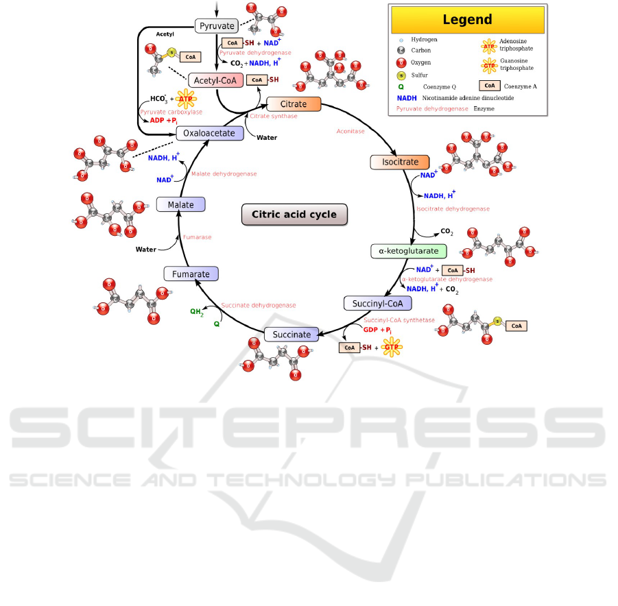
Figure 1: The Citric Acid Cycle (cf. Wikipedia: Narayanese, WikiUserPedia, YassineMrabet, TotoBaggins [GFDL
(www.gnu.org/copyleft/fdl.html) or CC BY-SA 3.0 (creativecommons.org/licenses/by-sa/3.0)], via Wikimedia Commons).
cess and of its underlying principles. We also describe
a pathway-modeling support layer (PMSL), which in-
cludes, among others a specification template. The
PMSL enables the modeling of new pathways in-
crementally and intuitively, one reaction at a time,
by specifying for each reaction its input substrates,
output products, facilitating enzyme, and a few con-
straints; i.e., required environmental conditions. The
PMSL also provides the automatic LSC code genera-
tion from template specifications.
The modeling method supports visualization of
the implemented reaction network at multiple levels.
The (static) specification’s live-sequence charts pro-
vide the reader with a procedural view of each re-
action. At run time (play-out), one can observe the
coordinated progression of all scenarios. And, after
the run, visualization of the simulation log enables
coarser-grain quantitative observation of the dynam-
ics of the system and of participating substances.
3.1 Related Modeling Techniques
Below we briefly review common techniques for
modeling metabolic pathways, including: Constraint-
Based Modeling (CBM) (see, e.g., (Becker et al.,
2007), Stochastic Simulation Algorithms (SSAs)
(see, e.g., (Gillespie, 1976)) and Rule-Based Model-
ing (RBM) (see, e.g., (Sneddon et al., 2011)).
CBM. CBM provides a numeric steady-state so-
lution for a set of ordinary differential equations that
fully describes a set of chemical reactions, includ-
ing influx and efflux exchange of chemical substances
between the system and its environment. (Schellen-
berger et al., 2011). CBM provides a quantitative, an-
alytic solution for the system’s steady-state composi-
tion but does not provide mechanistic modeling of the
reaction dynamics along the time axis.
SSAs. SSAs iteratively compute the quantitative
changes a system undergoes over time, assuming a
well-stirred, closed system at thermal equilibrium,
based on reaction-occurrence probabilities and reac-
tion rates derived from the theory of statistical ther-
modynamics. At each iteration, the model updates the
molecular quantities, as implied by the occurrence of
one reaction in an infinitesimal time interval.
The SSA method relies on initial quantities, on re-
action probabilities and on reaction rate constants. In
SSA, each reaction occurs as an atomic function, ac-
cording to its probability of occurrence. In nature,
there could be a situation where two reactions com-
pete for a common input substance. One reaction
binds an input molecule (say, of type S
1
), preventing
MODELSWARD 2019 - 7th International Conference on Model-Driven Engineering and Software Development
456

the use of this individual molecule by a competing re-
action that is active at the same time, and which may
have bound other input molecules (say, of type S
2
).
One of these reactions will be carried out successfully,
while the other (the second one in our example) will
either release the bound substance (of type S
2
), or be
delayed until another molecule of the necessary type
(S
1
) is available. In SSA, where reactions occur se-
rially, each one as complete unit of execution, whose
order is determined only by probability values, this
aspect of parallel chemical dynamics which compete
for common resources is not directly addressed. In-
stead, under some conditions reactions will occur if
and only if all inputs are available for binding. If an
input is missing the reaction halts and becomes a rate-
limiting factor in the metabolic pathway (and in the
simulation dynamics).
RBM. Rule-Based Modeling aims to handle the
obstacles of binding multiplicity, and the growing
combinatorial complexity in large biochemical sys-
tems. Additionally, it is aims to overcome the knowl-
edge gap between exact mechanistic solutions of
chemical reactions and the growing need for large-
scale calculations of biochemical systems, which may
lack the parameters needed for full analytic solution.
While both CBM and SSA provide quantita-
tive solutions without actually tracking individual
molecules as they (or their parts or atoms) become
parts of various substances, RBM differs from SSAs
in that it simulates reaction dynamics from the molec-
ular perspective. In RBM, each molecule is repre-
sented by a system object, which obeys to a set of
conditions (i.e., rules) over the molecule’s biochem-
ical reactivity. This enables molecular ID tracking
throughout the simulation.
BioNetGen is an RBM language used for model
specification (Faeder et al., 2009). As such, system
rules that apply to all molecular objects are possible
by time-dependent global functions. i.e., at a cer-
tain time point, the rule actions occur. This makes
the system rules independent of the system dynamics.
In contrast to CBM, SSA and RBM, scenario-based
modeling (SBM) enables time-dependent simulation
of a set of system reactions and conditions that apply
to the entire system simultaneously, while also capa-
ble of tracking individual molecules. SBM enables
dynamic allocation and deallocation of molecules by
the system’s scenarios. This allocation/deallocation
can be activated by a change in the system’s molecular
quantities, e.g., the elimination of a specific molecule
quantity can lead to allocation of a new molecule at a
desired quantity. Formation of a new substance can be
triggered by other molecules (namely, chained reac-
tions), by reaching a quantitative threshold of another
substance or, externally, by reaching a pre-determined
simulation time. In addition, global reaction guards
can be implemented in a way similar to other sim-
ulation scenarios. This enables formalization of in-
hibitory and regulatory biochemical reactions. SBM
enables reactive, time-dependent simulation, capable
of molecular tracking, and is not confined to equilib-
rium constraints. It combines the advantages of RBM
in terms of simulation time-dependency, molecular
tracking and coarse-grain approximations.
4 LSC MODELING OF
BIOCHEMICAL PATHWAYS
4.1 Individual Reaction Process
Fig. 2 represents a process, whereby an enzyme binds
a substrate (or multiple substrates) as well as co-
enzyme molecules, breaks certain chemical bonds and
forms others, and thus changes the substrates into
products. Soon after product formation, the bound as-
sembly of enzyme and products molecules separates
back into the solution, making all of them available
for further reactions
1
.
Biochemical reactions obey the following rules:
1. The substrates and the enzyme must be present
and available for binding. (At this point, we ig-
nore the aspect of spatial molecular proximity.)
2. Total substrate concentrations must be larger than
the total product concentrations. (In our model
we assume full diffusion and treat quantities, i.e.,
molecule counts, as equivalent to concentration.
There can be additional concentration/quantity-
related conditions that restrict specific reactions,
e.g., that the concentration of a particular output
product is significantly lower than that of a partic-
ular input substance.)
3. When binding occurs, the molecular components
involved become unavailable for further interac-
tions with the environment.
4. When all required conditions are met, an enzy-
matic complex is formed, and then turns into free
enzyme and products at a specific reaction rate.
4.2 Specifying Reaction Characteristics
A preliminary activity in modeling a pathway is
specifying all participating molecule types — i.e,
1
The biochemical concept of a by-product is treated here
as a product, and a co-enzyme is treated as an input substrate
that is also as an output product.
Using Reactive-System Modeling Techniques to Create Executable Models of Biochemical Pathways
457
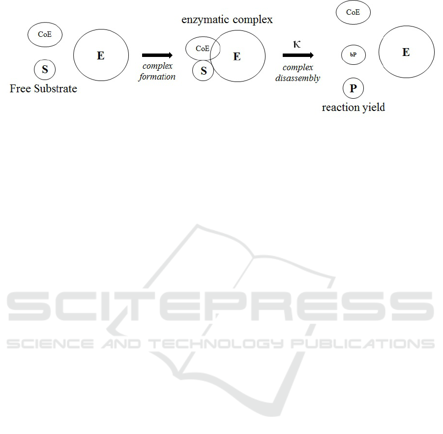
Figure 2: A schematic diagram of a biochemical reaction.
substrates, products, and enzymes — in the data
model. The PMSL provides a class named Molecule,
and the modeler specifies one object instance for
each molecule type (see Fig. 3). For example, the
substances appearing in the LSC in i.e., Citrate,
CisAconitate, H2O, and Aconitase appear as object
instances in the model. The Molecule class has an in-
teger attribute quantity for the number of molecules
of each molecule type, as well as common methods
for adding to and subtracting from this attribute.
Since there is a great similarity among the pro-
gressions and conditions of different reactions, the
PMSL provides a reaction-specification template,
which accommodates the biologist’s view, and from
which LSC specifications are generated automati-
cally. The template is coded in the form of a single
Java method call, createLine(rName,s1,s2,s3,
p1,p2,p3,p4,e,rRate) with the following reaction
parameters:
• rname: a reference name for the reaction; it will
become the name of the generated LSC.
• s1-s3: a list of up to three substrates
• p1-p4: a list of up to four products.
• e: the enzyme, and
• rRate: a reaction-rate parameter, relative to other
reactions in the model
For example, the method call createLine(Line1,
Citrate,,,CisAconitate,H2O,,,Aconitase,5) spec-
ifies the reaction commonly considered as the ‘first’
reaction in the cycle, where Citrate turns into
CisAconitate and water, with the mediation of the
Aconitase enzyme, during five (synthetic) time ticks.
The citric-acid cycle is classically comprised of
ten reactions. Three of these are associated with ad-
ditional reverse reactions, that is, ones that are sym-
metric to the ‘original’ forward reactions in that they
work with the same substances but in the opposite di-
rection: using the same enzyme, the substrate input
and the product output of the reverse reaction are, re-
spectively, the product output and substrate input of
the forward reaction. In our model, reverse reactions
are modeled as ordinary reactions. By convention,
we give them the same name as the forward reaction,
but with the letter R appended (yielding in our case
Line1R, Line2R, and line9R) (see Fig. 4).
The generic common conditions that are enforced
in all reaction LSCs generated by the PMSL include:
• MIN(S1,S2,S3) > MIN(P1,P2,P3,P4), where
S1-S3, and P1-P4 stand for the quantities of the
respective substances s1-s3 and p1-p4.
• MIN(S1,S2,S3) > 0, i.e., minimal quantities
must exist for each input substrate and
• E>0, i.e., at least one molecule of the enzyme e
must exist in the system.
Reaction-specific guards are presently coded man-
ually in the model, inside the createLine method,
associating with specific line names concise condi-
tions such as P
i
< a ∗ S
j
for a given constant a, the
quantity of a particular input S
j
, and the quantity of
a particular output, P
i
. Given the common structure
of these conditions, they can be added to the template
reaction method call in the future.
As part of the PMSL, the methods of the Molecule
class maintain an array for each molecule type, where
each array cell represents the availability and binding
status of individual molecules of this type.
When a scenario given by an LSC attempts to per-
form a particular reaction, it first calls the Molecule
class method lock, to acquire each concrete individ-
ual input molecule and enzyme required by the reac-
tion. If such a molecule exists, this is indicated by a
corresponding status in the array. If the reaction con-
cludes successfully, the quantities of some molecules
are decreased, and the corresponding array cells prac-
tically ‘disappear’. If the reaction is aborted, e.g.,
when some prerequisite conditions are not met, the
locked molecules are unlocked and become available
for future attempts of this and other reactions.
Upon successful completion of reactions, product
quantities are increased, and cells are added to the cor-
responding molecule- type arrays.
MODELSWARD 2019 - 7th International Conference on Model-Driven Engineering and Software Development
458
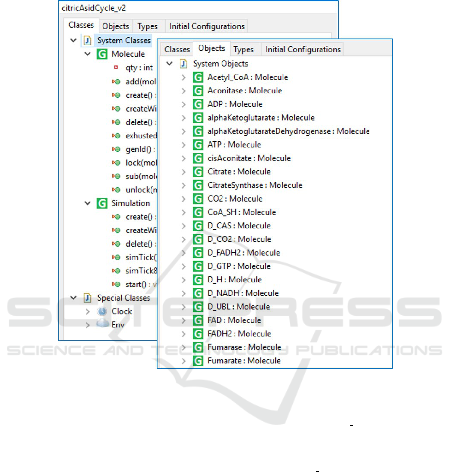
Figure 3: Definition of the Molecule class and its instances (the participating substances) in the PlayGo tool.
The locking function also marks the cell with a
unique reaction process id, so that when a reaction
attempt fails, all and only the molecules that were
locked by this particular attempt are released. This
indicator also enables seeing all the molecules associ-
ated with a given reaction instance at a given time.
Pathways are often circular, i.e., some outputs of
the ‘last’ reaction are inputs of the ‘first’ one. How-
ever, in reality, there must be a constant supply, i.e.,
sourcing, of certain input substances that are not pro-
duced by other reactions in the pathway, and removal,
or draining, of product substances that are not con-
sumed by reactions in this pathway. In the cell,
the sourcing supply often comes from the output of
other pathways (e.g., protons) or from the environ-
ment (e.g., water), and the drain is consumed by other
pathways (e.g., ATP), or is released into the environ-
ment (e.g., Carbon Dioxide).
In order to model an individual pathway, we
model Source and Drain reactions similarly to mod-
eling a general reaction using the reaction template.
Drain reactions are composed of an input substrate
and a dummy enzyme, ‘D name’. Upon reaction
activation, ‘D name’ binds the input and subtracts
its molecular quantity. Source reactions are speci-
fied with outputs, but with no inputs, again, using a
dummy enzyme, ‘S name’. Source and drain scenar-
ios are activated externally using a simulation time
trigger. In the future, these LSC scenarios can be
triggered also by the crossing of molecular quantity
thresholds or by other system conditions.
The LSC concept of a cold violation (see (Damm
and Harel, 2001)) is used to abort reactions when re-
action conditions are not satisfied.
After specifying all reactions as createLine()
method calls in the Java source file for each of the
reactions, the modeler compiles the file and runs the
resulting PMSL module. This generates an LSC for
each reaction (see, e.g., Fig. 5), and additional com-
mon LSCs, such as the ones triggering simulation
Using Reactive-System Modeling Techniques to Create Executable Models of Biochemical Pathways
459
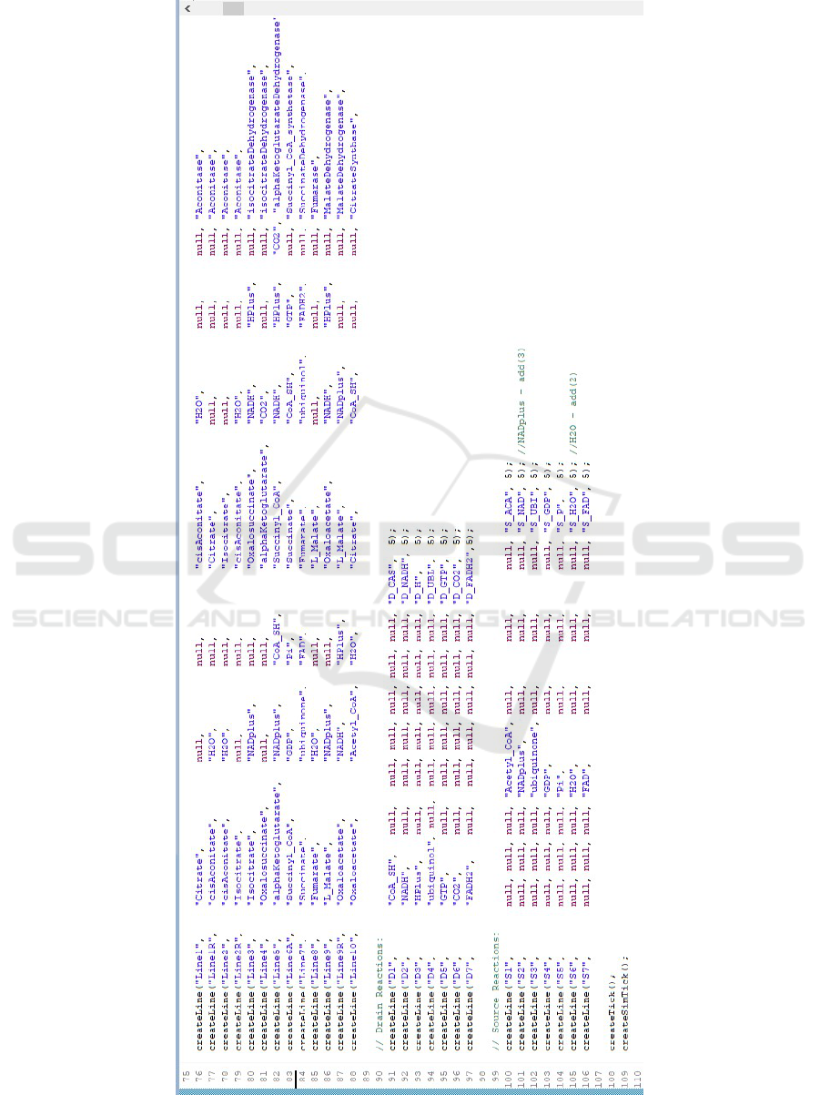
Figure 4: Specifying the citric-acid cycle in the PSML template.
MODELSWARD 2019 - 7th International Conference on Model-Driven Engineering and Software Development
460

clock ticks for coordinating reaction rates.
All scenarios are designed to be fully concur-
rent in order to more closely simulate the real-world
metabolic processes. Since in LSC semantics events
occur one at a time, the execution of scenarios is ac-
tually interwoven, rather than being fully concurrent.
A copy of each scenario begins whenever a simu-
lation time tick occurs. Unique identifiers for individ-
ual molecules of each kind are obtained, and these are
then locked. When no molecules exist to be locked,
an event exhausted is triggered. If this event occurs
out of order in any scenario it forces the main subchart
(scoped block) of the scenario to be exited, proceed-
ing with code that releases the obtained locks.
All reaction guards are then checked. If the condi-
tions are not met, again the subchart is exited and the
obtained locks are released.
When all guard conditions are met, substrate
quantities are subtracted. The reaction then waits for
the specified number of time ticks. Then, the quan-
tities of the reaction’s products are increased, and
the molecule array is internally adjusted to reflect the
availability of these new array cells, which represent
individual molecules. Finally, all remaining locked
molecules (e.g. enzyme) are released.
4.3 Flow Visualization
The simulation is run by playing out the
scenarios in PlayGo (see example video
at https://youtu.be/jPMggD6PoOg): all scenarios
are instantiated and synchronized; at a given synchro-
nization point, the composite system state (termed
the system cut), is implied by the current state (cut)
of each of the scenarios, which, in turn, is implied
by the currently-active location in each lifeline of
the scenario. When an event occurs, all affected
scenarios make their respective transitions, resulting
in a new system cut.
As part of the pathway simulation infrastructure
the system produces an event log. With every key
event, like add and sub, an event-log record is writ-
ten to an external file. The file is then used for pro-
ducing dynamic quantity and state visualization (us-
ing the Python FFmpeg package), as shown in Fig. 6
and in the second part of the above video.
The upper panel shows LSCs activity: the hori-
zontal axis represents the ten citric-acid cycle reac-
tion scenarios; the vertical axis represents each sce-
nario’s progress; ‘positive’ bars (above idle level)
represent forward-reactions activity (substrate lock
or subtract, or product add); ‘negative’ bars (be-
low idle level) represent progress of the reverse re-
actions. Note that during execution the simulation en-
gine treats all reactions in the same way and, in par-
ticular, it does not distinguish between forward and
reverse reactions. The distinction in the visualization
relies purely on the naming convention we applied.
The bottom panels in Fig. 6 represent the molecu-
lar quantities, and provide the user with a quantitative
sense of the progress of the system’s behavior. For
convenience, and specifically for this application, we
have separated all the molecular substances partici-
pating in the cycle into three groups: inputs, interme-
diate products and outputs.
The simulation starts with only input molecules.
During a run, one can observe how progress of the
LSCs adds intermediate molecular products. Eventu-
ally, the system accumulates output products. When
source and drain reactions are not modeled, at some
point, the system runs out of required inputs and is
jammed with products. When source and drain are
added, at the appropriate reaction rate, the reactions
should, in principle, proceed indefinitely (see, e.g.,
the demonstration movie).
5 PATHWAY
INTERCONNECTION
So far, we have discussed a single model, including
the ten basic reactions of the citric-acid cycle, the
three reverse reactions, and the source and drain re-
action. Clearly this principle can be applied to other
pathways.
Of particular interest is the connection of two sep-
arate pathways. Consider, for example, the Pyruvate
cycle attached to the main citric-acid cycle (see top
left part of fig 1). This cycle produces some of the
inputs consumed by the citric-acid cycle, modeled
above as source reactions. Conversely, some sub-
stances produced by drain reactions of the Pyruvate
cycle are consumed as inputs of the Citric-acid cy-
cle. When modeling the two cycles together, one
needs to simply include the reactions of both in a
single sequence of createLine() specifications, re-
move source and drain reactions that become redun-
dant in this composition, adjust the reaction rates into
a common relative scale and provide quantitative up-
date to the initial conditions of the system molecules.
6 DISCUSSION AND FUTURE
WORK
We have demonstrated an initial, yet readily general-
izable, approach for modeling biochemical pathways,
Using Reactive-System Modeling Techniques to Create Executable Models of Biochemical Pathways
461
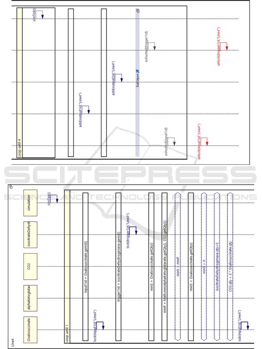
Figure 5: An LSC for a Krebs cycle reaction.
MODELSWARD 2019 - 7th International Conference on Model-Driven Engineering and Software Development
462
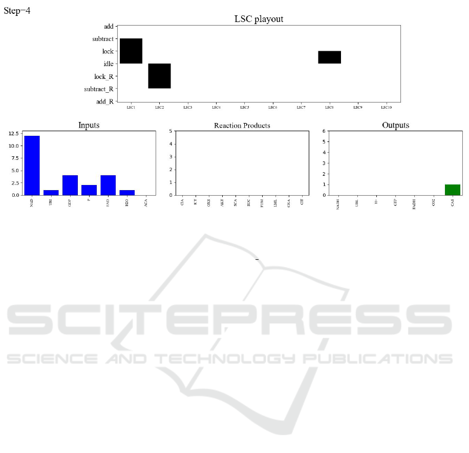
Figure 6: Simulation visualization snapshot. The top panel depicts the current state of each of the ten reaction LSCs
listed on the X axis. The Y axis shows each reaction’s progression: from idle to lock— locking enzyme and substrates,
to subtract—reducing quantities of inputs, to add—increasing output quantities. Reverse reactions occupy the same X-
axis location as their forward counterpart with Y-axis states marked R, below the idle state. The bottom panel tracks the
quantities of substances: initial inputs, intermediate reaction products and outputs that must be drained. The figure captures
the run relatively early, hence most of the inputs are still available (only ACA was depleted), and only one product (CAS) has
been produced. The intermediate-product chart is empty, since the ones that were produced were already consumed.
characterized by the following properties:
Incrementality. The scenarios for the various re-
actions exist in the specification ‘side-by-side’, with-
out directly referencing each other. More reactions
can be added in the same manner, when new discov-
eries and/or refinements are made, or to model inter-
action with other pathways.
Clarity. First, each scenario on its own depicts
in a readily-understandable way the main aspects of
what is known to happen in a reaction. Additional
aspects can be added within the scenario or in separate
ones. Second, concise specification of the entire cycle
in only a few lines further facilitates mental grasping
of the orchestrated operation of the pathway.
Generality of Constraints. The LSC language
enables programming, separately, essentially any con-
straint (Turing-computable, of course) that a sys-
tem can impose on any of its components. System
constraints can be implemented inside an ordinary
(pathway-specific) LSC, or in the reaction template
that translates to LSCs. Each such constraint can then
affect all LSCs without the need to explicitly specify
direct LSC-to-LSC communication. This flexibility is
not normally available in modeling methods.
Ease of Conceptualization. The inter-
dependencies between biochemical reactions are
embedded in the compositional semantics of the
underlying LSC language; i.e., parallel execution of
multiple reactions, repeated synchronization, trigger-
ing of events that are requested and not blocked, etc.
Once these general principles are understood, the
pathway-specific dependencies are easily understood
implicitly, without the need to depict them explicitly.
That is, there are no especially constructed connec-
tors between LSCs that depict such composition and
dependencies. We believe that combined with the
intuitive syntax of individual LSCs (and, of course,
of the reaction template), this enables the formation
of a cognitive representation of how a particular
biochemical pathway works, and, moreover, it makes
it possible to understand the principles that drive
similar pathways.
Ease of Visualization. The abstraction of com-
plex behaviors as a sequence of events enables the
creation of process visualizations over multiple di-
mensions (some of which were shown above): pro-
gram progression and state changes, quantitative de-
piction, tracing the state of a particular molecule or
set thereof, etc.
Additional research and development is needed
in several areas: (i) A wide variety of pathways
need to be modeled in order to more deeply demon-
strate the commonality and generality of the princi-
ples of the approach; (ii) multiple pathways should
be combined in a single model to demonstrate SBM
modeling of complex networks; (iii) empirical stud-
Using Reactive-System Modeling Techniques to Create Executable Models of Biochemical Pathways
463

ies with human-observable measures are needed, to
more rigorously substantiate the claim that human au-
diences indeed benefit from the approach; (iv) the
model should be extended to accommodate multiple
instances of scenarios, each instance working (in par-
allel) on a different set of molecule instances; (v) the
reaction rates should be enhanced, and reaction prob-
abilities added to the reaction LSCs; (vi) following
the above (and depending on their success), physi-
cal spatial location attributes and a diffusion model
should be added to the molecules; (vii) the scalabil-
ity of the system should be enhanced to support much
larger quantities.
7 CONCLUSION
We have shown that the scenario-based approach to
modeling can be successfully applied in the domain
of modeling and simulating biochemical pathways.
We have argued that it offers capabilities that seem
promising in the learning process of students, and
in improving the ability of various audiences to un-
derstand specific biochemical pathway dynamics, and
biochemistry concepts in general.
ACKNOWLEDGEMENT
This research was supported by grants from the the
German-Israeli Foundation for Scientific Research
(GIF), The Minerva Foundation and the Israel Science
Foundation (ISF).
REFERENCES
Becker, S., Feist, A., Mo, M., Hannum, G., Palsson, B.,
and Herrgard, M. (2007). Quantitative prediction of
cellular metabolism with constraint-based models: the
cobra toolbox. Nature protocols, 2(3):727.
Damm, W. and Harel, D. (2001). LSCs: Breathing life into
message sequence charts. J. on Formal Methods in
System Design, 19(1):45–80.
Faeder, J., Blinov, M., and Hlavacek, W. (2009). Rule-based
modeling of biochemical systems with bionetgen. In
Systems biology, pages 113–167. Springer.
Gillespie, D. (1976). A general method for numerically
simulating the stochastic time evolution of coupled
chemical reactions. Journal of computational physics,
22(4):403–434.
Gordon, M., Marron, A., and Meerbaum-Salant, O. (2012).
Spaghetti for the main course? observations on natu-
ralness of scenario-based programming. 17th Annual
Conference on Innovation and Technology in Com-
puter Science Education.
Harel, D., Kantor, A., Katz, G., Marron, A., Mizrahi, L.,
and Weiss, G. (2013). On composing and proving cor-
rectness of reactive behavior. EMSOFT.
Harel, D., Katz, G., Lampert, R., Marron, A., and Weiss, G.
(2015). On the succinctness of idioms for concurrent
programming. In Proc. 26th Int. Conf. on Concur-
rency Theory (CONCUR), Madrid, Spain.
Harel, D., Maoz, S., Szekely, S., and Barkan, D. (2010).
PlayGo: towards a comprehensive tool for scenario
based programming. In ASE.
Harel, D. and Marelly, R. (2003). Come, Let’s Play:
Scenario-Based Programming Using LSCs and the
Play-Engine. Springer.
Harel, D., Marron, A., and Weiss, G. (2012). Behav-
ioral programming. Communications of the ACM,
55(7):90–100.
Kam, N., Kugler, H., Marelly, R., Appleby, L., Fisher, J.,
Pnueli, A., Harel, D., Stern, M., and Hubbard, E.
(2008). A scenario-based approach to modeling devel-
opment: A prototype model of c. elegans vulval fate
specification. Developmental biology, 323(1):1–5.
Marron, A., Hacohen, Y., Harel, D., M
¨
ulder, A., and Ter-
floth, A. (2018). Embedding Scenario-based Model-
ing in Statecharts. In Model-driven Robot Software
Engineering workshop (MORSE), in MoDELS.
Schellenberger, J., Que, R., Fleming, R., Thiele, I., Orth,
J., Feist, A. M., Zielinski, D., Bordbar, A., Lewis, N.,
Rahmanian, S., et al. (2011). Quantitative prediction
of cellular metabolism with constraint-based models:
the cobra toolbox v2. 0. Nature protocols, 6(9):1290.
Sneddon, M., Faeder, J., and Emonet, T. (2011). Efficient
modeling, simulation and coarse-graining of biologi-
cal complexity with nfsim. Nature methods, 8(2):177.
MODELSWARD 2019 - 7th International Conference on Model-Driven Engineering and Software Development
464
