Robust Fitting of Geometric Primitives on LiDAR Data

Tekla T

oth and Levente Hajder

Department of Algorithm and Applications, E

otv

os Lor

and University,

Pazmany Peter stny. 1/C, Budapest 1117, Hungary

Keywords:

Surface Fitting, Geometric Primitives, Light Detection and Ranging, Robust Fitting.

Abstract:

This paper deals with robust surface ﬁtting on spatial points measured by a LiDAR device. The point clouds

contain hundreds of thousands data points. Therefore, the time demand of the algorithms is crucial for fast

operation. We present two novel algorithms based on the RANSAC method: one for plane detection and

one for other object detection. The execution time of the novel algorithms is signiﬁcantly lower as only one

random sampling is required because a deterministic teqnique selects the other data points. The accuracy of

the novel methods are validated on synthesized data as well as real indoor and outdoor measurements.

1 INTRODUCTION

3D vision (Hartley and Zisserman, 2003) is one of

the most challenging research topic of computer sci-

ence. There are many different sensors for machine

perception systems that can produce accurate spatial

data from our 3D world. Vision applications are usu-

ally based on digital cameras. However, other sensors

become popular recently.

The aim of this paper is to show that LiDAR

(Light Detection And Ranging) technology can be ef-

fectively used for 3D object detection. It is a survey-

ing method that measures distance to a target by illu-

minating the target with pulsed laser light and measur-

ing the reﬂected pulses with a sensor. Differences in

laser return times and wavelengths can then be used to

create digital 3-D representations of the target. (Deﬁ-

nition of LiDAR is from Wikipedia (TM)).

It is demonstrated in this paper that the accuracy

of a LiDAR scans is enough to detect geometric prim-

itives such as planes, spheres and cylinders. The for-

mer and the latter ones are especially important ob-

jects as they usually appear in real-world scenes: the

ground and the walls of the buildings are planes, and

advertising columns and lamp posts form cylinders.

The challenge of 3D object ﬁtting algorithms is

that LiDAR devices can scan only one side of the

object, because more than half of the objects are oc-

cluded.

1.1 Related Work

Fitting geometric primitives on LiDAR point clouds is

a relatively new research topic. The main idea here is

to adapt efﬁcient ﬁtting methods to point clouds taken

by LiDAR devices.

This paper deals with the ﬁtting of planes, spheres

and cylinders. The latter two tasks are more challeng-

ing as only part of the object can be measured due to

self-occlusion. Plane ﬁtting seems to be signiﬁcantly

simpler, but this task can be speeded up if specialties

of urban scenes are considered.

Plane Fitting. LiDAR technology has become

popular for the last decade although the price of the

devices are quite high. To the best of our knowledge,

the ﬁrst solved task using LiDAR was the plane

ﬁtting (Tsai et al., 2010) which is a long-time

researched problem in 3D geometry with efﬁcient

solutions (Pratt, 1987; Eberly, c; Eberly, b). Detected

planes can be used for several purposes, e.g. motion

registration (Grant et al., 2013) or reconstruction of

buildings via roof detection (Awrangjeb and Fraser,

2014).

Sphere Fitting. Although spheres are relatively sim-

ple geometric objects that can be reconstructed efﬁ-

ciently (Eberly, c), the detection of spheres on Li-

DAR data is not frequently addressed, maybe because

spheres do not usually appear in urban environment.

However, (Pereira et al., 2016) showed that spheres

are very useful for registering different point clouds,

taken by LiDAR devices, into a common system.

622

Tóth, T. and Hajder, L.

Robust Fitting of Geometric Primitives on LiDAR Data.

DOI: 10.5220/0007572606220629

In Proceedings of the 14th International Joint Conference on Computer Vision, Imaging and Computer Graphics Theory and Applications (VISIGRAPP 2019), pages 622-629

ISBN: 978-989-758-354-4

Cylinder Fitting. Cylinder ﬁtting (Eberly, a) is more

challenging than reconstruction of spheres, neverthe-

less, advertising columns often appear in large cities,

therefore cylinder ﬁtting is a realistic problem for

machine perception. To the best of our knowledge,

cylinder ﬁtting is addressed only on laser scanned

data (Nurunnabi and andoderik Lindenbergh, 2017).

In this paper, we show how planes, spheres, and

cylinders can be reconstructed from LiDAR point

clouds. The main challenge of these problems is that

only part of the observed object is visible due to self-

occlusion. The contributions of our paper are as fol-

lows: (i) a novel modiﬁcation of RANSAC algorithm

is introduced for robust plane ﬁtting; another similar

modiﬁcation is applied for sphere and cylinder ﬁtting.

(ii) The appendix contains basic and precise geomet-

ric methods for plane, sphere and cylinder ﬁtting that

can yield accurate object parameters even if the meth-

ods are supported by LiDAR data; (iii) The efﬁciency

of the methods are validated both on synthesized and

real data-world data.

2 PROPOSED METHODS

In this section, we introduce novel robust ﬁtting meth-

ods. Development issues are also discussed here.

2.1 Robust Model Estimation

Our shape detection is based on RANSAC (Fischler

and Bolles, 1981) (RAndom SAmpling Consensus)

algorithm. RANSAC is a method which ﬁts a model

from randomly sampled subset of an observed dataset.

It works with arbitrary model. For line ﬁtting, the

basic steps of the RANSAC algorithm is visualized in

Figure 1. These are as follows:

1. Randomly select a subset from the original

dataset. Usually, the size of the subset is the min-

imal one. For example, two/three points are se-

lected for line/plane ﬁtting.

2. Model is ﬁtted to the selected subset.

3. Classiﬁcation of all the points of the dataset to

inliers/outliers based on an error function. For

line/ﬁtting, a point is an inlier if it is closer to the

line/plane than a given threshold. It is a disadvan-

tage of the method that this threshold is usually

given empirically. The set of inliers is called con-

sensus set..

4. The estimated model is accepted if the consensus

set is large enough.

5. Modiﬁcation of the accepted model by reﬁtting it

from the inliers.

(a) Step 1 (b) Step 2 (c) Step 3 (d) Step 4-

(e) Step 6

Figure 1: Illustration of RANSAC algorithm for line ﬁtting.

The titles of the subﬁgures denote the steps of the algorithm.

6. Repeat steps 1-5 several times. Repetition number

can be calculated if outlier ratio is approximately

known. If we reach one or more successfully ﬁtted

results, the model with the largest consensus set is

chosen.

RANSAC is a reliable method. However, for

multi-model ﬁtting it is not a viable solution as the

number of iterations is extremely high if only a small

portion of the data points belong to an object. Table 1

shows the required number of iterations. Remark that

at least three data points are necessary for plane and

cylinder ﬁtting, while spheres require more than that.

If only ﬁve percent of the dataset corresponds to

a plane, more than 36.000 iterations are required to

obtain good result with 99% probability. It is very

time-consuming even if GPU is applied for the com-

putation.

2.1.1 Plane Detection

The original algorithm can be parallelized to make it

faster, but there are several properties in case of Li-

DAR point clouds which can improve the algorithm.

Our modiﬁed RANSAC algorithm of plane detection

is based on two observations.

Observation 1. The planes in urban environment are

principally the ground or the walls of the buildings,

hence they contain a huge amount of points, up to half

of the whole cloud. Therefore, one can reduce the

search time with sampling, and we can construct a

more focused detection algorithm.

Table 1: Number of iterations required for original

RANSAC (Fischler and Bolles, 1981) algorithm if conﬁ-

dence is set to 99%. N denotes the number of sample points.

Both plane and cylinder ﬁtting requires at least 3 points. For

sphere ﬁtting, the minimum number is 4. Columns are vary-

ing w.r.t. outlier ratio from 50% to 95%. It is well seen that

N = 1 case is drastically faster than the others.

N 50% 65% 80% 90% 95%

1 7 11 20 44 90

3 35 106 573 4602 ∼ 10

4 72 305 2875 ∼ 10

∼ 10

Observation 2. The normal vectors of the planes are

usually either vertical or horizontal. With minimal

Robust Fitting of Geometric Primitives on LiDAR Data

623

Figure 2: Synthetic point generation and the planes along

the synthetic directions, yielding sets Ω

(green), Ω

(blue),

Ω

(red).

rotation can be reached that the planes are parallel to

two of the three coordinate axes.

Instead of taking a subset of sampling points, we

choose only one point P = (p

, p

) of the origi-

nal set. Four synthetic points are calculated along the

three planes perpendicular to the axes of the coordi-

nate system with a given t distance in the following

way, yielding point sets Ω

, Ω

, and Ω

Ω

= {(p

, p

), (p

, p

+t, p

+t), (p

, p

+t, p

−t),

, p

−t, p

+t), (p

, p

−t, p

−t)}

Ω

= {(p

, p

), (p

+t, p

, p

+t), (p

+t, p

, p

−t),

−t, p

, p

+t), (p

−t, p

, p

−t)}

Ω

= {(p

, p

), (p

+t, p

), (p

+t, p

−t, p

), (p

−t, p

)}.

(1)

This calculation is illustrated in Figure 2. Assume

that the red, green and blue colors denote axes X, Y

and Z. In the ﬁgure, the coordinates of point P is

(0, 0, 2), and the distance threshold parameter is set

to t = 2. The synthetic points of Ω

, Ω

and Ω

are

the middle point of the edges: there are four green,

four blue and four red points.

The input points of the plane ﬁtting algorithm are

the closest real points in the pointcloud to the syn-

thetic points. Point P is unchanged, but the other four

points are replaced for the closest one in the whole

pointcloud. We evaluate the minimal needed distance

from P during the tests. Furthermore, if the plane

searching parameter is t, the algorithm can detect the

planes, rectangles with area least t

After searching the closest real points, one can ﬁt

the planes to Ω

, Ω

and Ω

sets. Thus the three prin-

cipal planes, drawn by red, blue, and green in the ﬁg-

ure, are separately processed, they obtain three differ-

ent candidate planes. Then the consensus set of all the

planes is collected similarly to the original RANSAC

algorithm.

2.1.2 Sphere and Cylinder Detection

In case of a sphere or a cylinder, we can use a sim-

ilarly modiﬁed RANSAC algorithm. However, the

result depends on more parameters. After plane de-

tection, the remaining surfaces are built from partly

Figure 3: Estimation of the sphere center. Each candidate

point pair of the sphere determines a plane. The sphere cen-

ter is the intersections of these planes.

covered but continuous pointsets and they are easily

separable in space. Hence the search to ﬁnd the can-

didate spherical and cylindrical objects can run in par-

allel. The algorithm randomly chooses a single point

and takes the closest points within a predeﬁned dis-

tance. The inliers are the points with neighboring

point which Euclidean distance is smaller than a given

threshold parameter t. When the pointset contains less

then k points, it is discarded. k are set in an empirical

way, see the test section for our setting. Then the sur-

face ﬁtting is carried out on the selected points, yield-

ing a candidate model. The further steps are similar

to the original RANSAC. The ﬁnal model contains the

most inliers.

2.2 Surface Fitting Methods

The main goal is to detect planes, spheres and cylin-

ders from noise point clouds, therefore very effective

and robust ﬁtting algorithms are needed. We suggest

efﬁcient ﬁtting methods, the suggested algorithms are

written in the Appendix in detail. However, in case of

the LiDAR data, we have to modify the algorithms,

because of the special properties of the LiDAR point

clouds. The following two subsection introduce our

new methods for sphere and cylinder ﬁtting.

Estimation of the Center of a Sphere. A good es-

timation for the center of the sphere is the average of

the sample points, as it is discussed in the appendix if

the surface of the sphere is uniformly sampled. How-

ever, this is a bad approximation in case of LiDAR

data where only one segment of the sphere is known,

because this solution needs too many iterations.

We implemented our method based on a geomet-

rical approach, which is visualized in Figure 3. The

center of the sphere can be estimated from the equa-

tions of its four points. Bisecting plane of two points

contains the center itself, and the intersection of three

bisecting planes is a good estimation for the center.

To our experience, 10 points are enough to select

because synthetic tests showed that it is an accurate

VISAPP 2019 - 14th International Conference on Computer Vision Theory and Applications

624

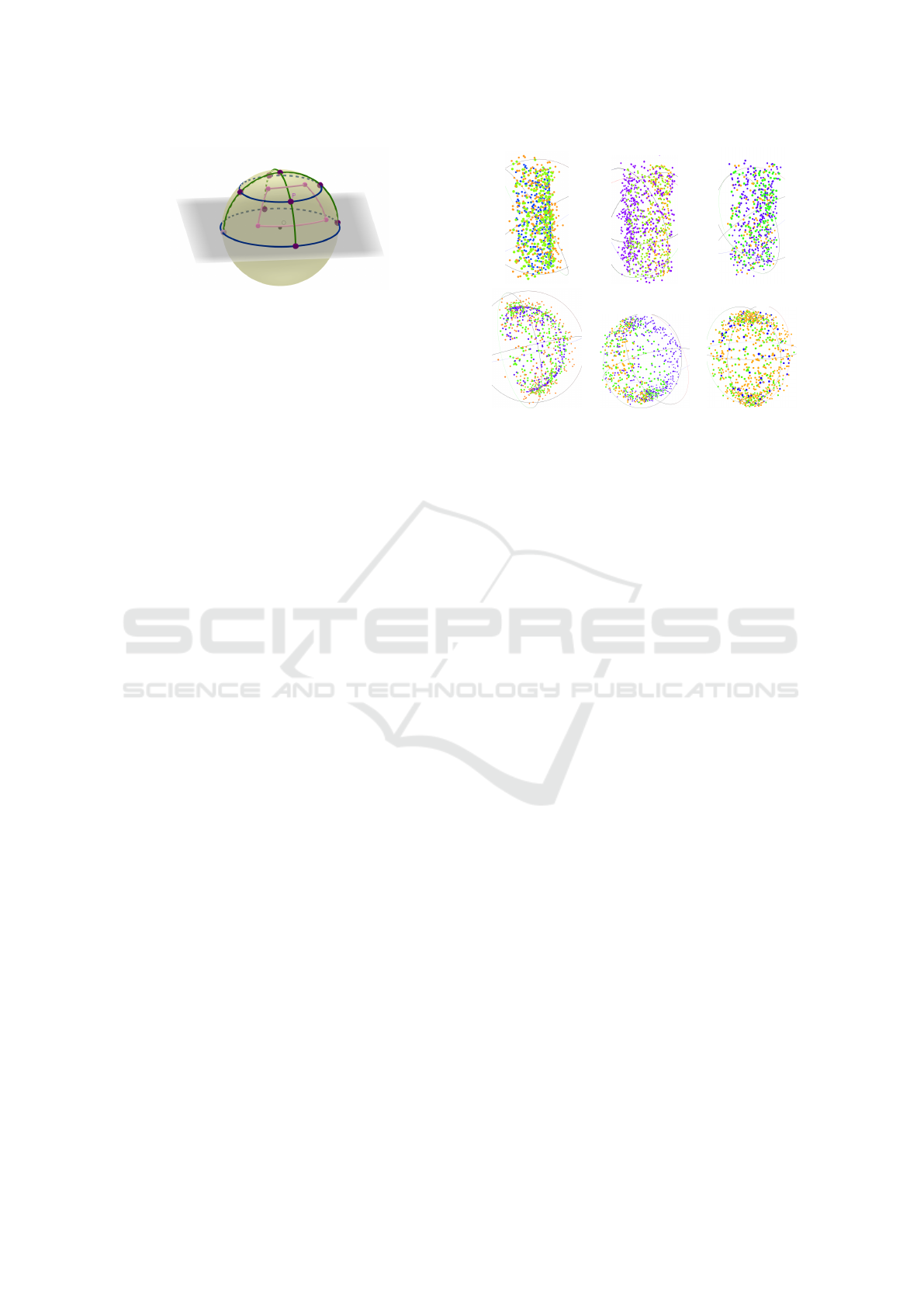
Figure 4: Hemisphere of the possible directions of the cylin-

der. The initial step evaluates the errors at the purple points.

Pink points denote the directions after bisecting the initial

intervals.

estimation, and more points yield increased computa-

tion time. Hence when there is a larger input pointset,

one can get a good estimation using 10 randomly cho-

sen points. After this, the ﬁxpoint-iteration gives the

local optimal solution.

Estimation of the Direction of the Cylinder. To

estimate the direction of the cylinder axis, we repre-

sent vector W with a two dimensional parameter. Vec-

tor W with spherical coordinates is given by Equation

4. The original method, written in the appendix, ﬁnds

this vector by exhaustive search. It splits the interval

of the two parameters into 1024 and 512 equal parts.

This gives a very accurate result because of the ﬁne

sampling.

However, most of the calculations are unneces-

sary. To reach the same result, an incremental approx-

imation is applied, yielding signiﬁcantly less time de-

mand. Figure 4 shows the initial step of the method,

where the hemisphere represents the set of the possi-

ble unit length directional vectors. At ﬁrst, we cal-

culate the ﬁtting error in the nine directions denoted

by the purple points, which are obtained by the equal

partitioning of the intervals of θ

and θ

into 4 and 3

parts, respectively. If the direction of minimal error

value is the labeled by point P, the optimal direction

is located within the pink part of the sphere. There-

after we iteratively bisect the intervals of θ

and θ

until the desired accuracy is reached.

3 TESTS AND RESULTS

The proposed algorithms are implemented in MAT-

LAB. The methods are tested both on synthetic and

real LiDAR datasets. The synthetic tests and indoor

data, measured by Velodyne HDL-64 and Velodyne

VLP-16-LiDAR, are made for sphere and cylinder ﬁt-

ting, and the outdoor data is designed to ﬁt planes and

cylinders.

Figure 5: Synthetic datapoints for cylinder (up) and sphere

ﬁtting (down). Left: Noise added to points. Middle: Oc-

cluded points removed. Right: pointset made sparser. In the

ﬁgures, blue dots represent original pointset, green when

the noise/point removing is moderate, yellow when high

amount of noise/point removing is applied. Best viewed in

color.

3.1 Test Data

The synthetic tests contain randomly generated points

of a plane, sphere or cylinder with given parameters.

The results were observed in the presence of growing

noise, occlusion and the number of the sample points.

The real tests are indoor and outdoor LiDAR mea-

surements. The difﬁculty is, that the HDL-64 data is

very noisy, and the outdoor data is only available with

this device, which was equipped on a car. The in-

door tests were made in a room with exact test objects,

however, the scene were fully continuous against the

street tests.

3.2 Synthetic Tests

In order to quantitatively test the robust ﬁtting meth-

ods, synthetic test sequences are generated. The main

goal for the test generation is to simulate the real mea-

surement. For this reason, three parameters can be

changed in our environment:

1. Noise. LiDAR technology has been improved

for the last decade, yielding more accurate mea-

surements. The precision of Velodyne HDL-64

is approximately 100 mm, that of VLP-16 is a

bit smaller. Remark that Velodyne VLP-16 is the

newer technology.

2. Occlusion. Normally, 3D scanning by a LiDAR

device can measure only one side of an object due

to self-occlusion. This effect can also be simu-

lated in our testing environment.

Robust Fitting of Geometric Primitives on LiDAR Data

625

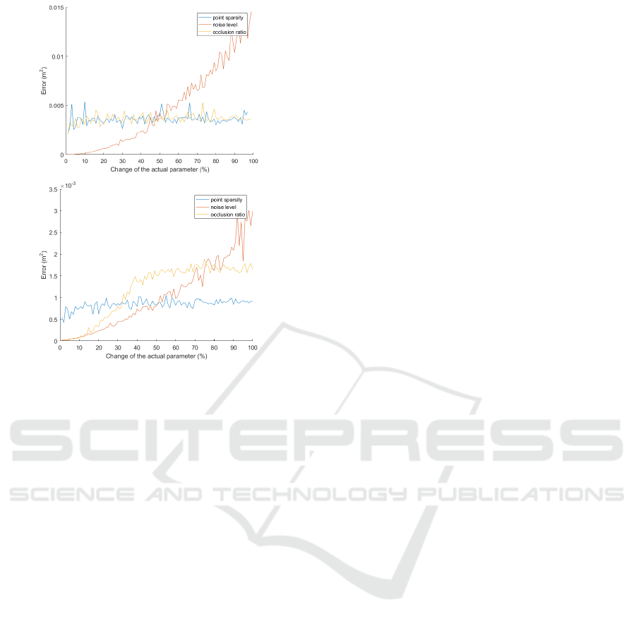
Figure 6: Error of sphere (top) and cylinder (bottom) ﬁt-

ting. Data are synthetically generated. Red, yellow, and

blue curves are noise level, occlusion ratio, and point spar-

sity, respectively. Vertical axis shows the ﬁtting error. Best

viewed in color.

3. Density of the Point Cloud. For real measure-

ment, density is determined by the applied LiDAR

device. It mainly depends on the number of the

beams. E.g. Velodyne HDL-64 and VLP-16 have

64, and 16 beams, the point cloud measured by

the former one is signiﬁcantly denser.

For the synthesized tests, a sphere with 0.375 m

radius, and a cylinder with 1.3 m height and 0.35 m

radius are generated. The ﬁtting of the two objects are

separately tested. The objects are translated in order

to make them viewable from the location of the syn-

thesized LiDAR. The object is rotated as well, how-

ever, it does not inﬂuence the sphere ﬁtting as spheres

are rotational symmetric.

Then noise is added to all the points in order to

simulate the measurement noise of the LiDAR tech-

nique. Finally, points are removed to simulate self-

occlusion and measurement by sparse devices. The

synthesized spheres and cylinders are visualized in

Figure 5.

Test results are plotted in Figure 6. The three

different test types are visualized in the same chart.

They are distinguished by different colors.

The tests show that the ﬁtting quality is principally

based on noise in both cases as the error increases

monotonically. The inﬂuence of the self-occlusion is

not signiﬁcant, but the sparsity of the point cloud af-

fects the results of the cylinder. These tests are run

100 times because of the random parameters, and the

same results are obtained.

As it is expected, the error is increasing in all test

cases: it is evident that noise, self-occlusion and point

removal make a ﬁtting less accurate.

3.3 Real Indoor Tests

The ﬁtting methods are tested on point clouds taken

in both indoor and outdoor environment. The indoor

tests are discussed ﬁrst. Some examples for sphere

and cylinder ﬁtting are shown in Figure 7 and 8.

An important task of the experiments is to tune

the free parameters of the algorithms on real datasets.

In case of plane detection, it is observed that if the

distance between the real point and the one generated

by the proposed method is less or equal than 5 cm,

the result becomes inaccurate. Furthermore, the op-

timal value of t is between 0.3 and 0.5 m, hence the

algorithm detects planes with dimensions greater than

[0.6×0.6]−[1.0 ×1.0]m. The plane detector requires

some trade-offs near the line where two planes cut

each oder. The ﬁrst time detected plane contains all

points inside the threshold t from both planes. So if t

is higher, the ﬁtting is very inaccurate, but if t is lower,

many good points are lost. For practical reasons, we

implemented a re-selection of the points near these

cutting lines.

The improved RANSAC needs less iterations, be-

cause it has to select only a single point from a plane,

the other four points are generated synthetically. If

we run the algorithms with the same iteration num-

ber, the modiﬁed algorithm selects the greatest plane

more times, so we get more accurate result.

The parameter t is set to 0.4 m in case of sphere

and cylinder ﬁtting, because real tests contains cylin-

ders with 1 − 2 m height. The minimal number of

points (k) is 15, because it approaches the expected

ﬁtting. Moreover, the improved sphere ﬁtting algo-

rithm needs one ﬁfth of the iterations to reach the

same sphere parameters as the original method.

3.4 Real Outdoor Tests

Outdoor tests are taken to test the plane and cylin-

der ﬁtting algorithm. There are many planes in urban

environment: the ground, building walls, side of vehi-

cles, etc. Cylinders also appear near the roads: adver-

tising columns can be modeled as regular cylinders.

Unfortunately, sphere testing is missing in the case

of outdoor testing as regular spheres do not appear in

cities to the best of our knowledge.

VISAPP 2019 - 14th International Conference on Computer Vision Theory and Applications

626

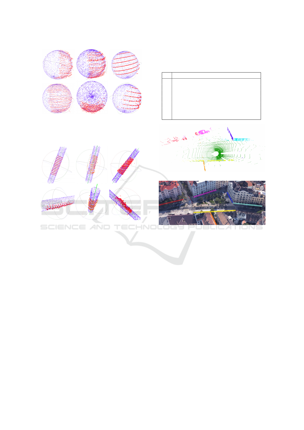
Figure 7: Fitted spheres. Point clouds in the left two

columns were taken by Velodyne HDL-64, right columns

by VLP-16. Red and blue dots visualize the measured and

ﬁtted data, respectively. The self-occlusion is the highest in

the middle column.

Figure 8: Fitted cylinders. Point clouds in the right two

columns were taken by Velodyne HDL-64, left columns by

16. Red and blue dots visualize the measured and ﬁtted

data, respectively. The self-occlusion is the highest in the

middle.

Figure 9 shows an example for plane ﬁtting. The

point cloud is taken in a crossroads where ﬁve verti-

cal walls around the measuring device. All of them

are successfully segmented. They are plotted by dif-

ferent colors in the ﬁgure. Table 2 consists of the time

demand, in seconds, of the original RANSAC and our

modiﬁed algorithm on this test scenario.

There are challenges even for plane ﬁtting: disad-

vantage of noisy points is demonstrated in Figure 10,

where the points of the same plane form different

quasi-parallel planes because of the mirroring of the

widows. It seems to impossible to ﬁlter out these

planes, because they really create false planes in the

pointcloud. The obtained plane parameters of this ex-

ample are shown in Table 3.

Geometrically, advertising columns or lamp posts

are cylinders. However, the number of the points cor-

responding to this objects are not too high. Real ex-

amples for cylinder ﬁtting is visualized in Figure 11,

the obtained parameters are listed in Table 4.

Table 2: Time demand of the plane detectors. T

original

and

proposed

denote the original RANSAC and the proposed

algorithm. Test results are visualized in Figure 9. Tests

were run 1000-times and average values are listed.

color N T

original

proposed

1. green 52857 16.434 17.945

2. yellow 4904 10.323 9.675

3. red 2239 8.932 7.830

4. light blue 2101 7.525 7.333

5. dark blue 1866 7.292 6.752

6. magenta 1518 7.043 6.425

7. orange 1344 6.992 6.182

(a) Outdoor measurement

(b) Real environment

Figure 9: The ﬁgure shows the similarity between the ﬁtted

planes to an outdoor measurement, and the map of the real

environment. Best viewed in color.

4 CONCLUSION

The paper proposes novel ﬁtting algorithms which

can reconstruct sphere, cylinder and plane. The goal

was to detect and reconstruct the given objects in a

sparse pointcloud.

The ﬁtting algorithms are efﬁcient and fast. The

RANSAC algorithm is modiﬁed to get fewer itera-

tion, decreasing the time demand. This modiﬁcation

is based on some special properties of the sparse point

cloud taken of urban environments.

The methods are tested on synthetic point clouds,

varying the amount of noise, the number of the points

and the self-occlusion. Real indoor and outdoor test

results are also presented, the advantages and limits

of the algorithms are discussed.

Robust Fitting of Geometric Primitives on LiDAR Data

627

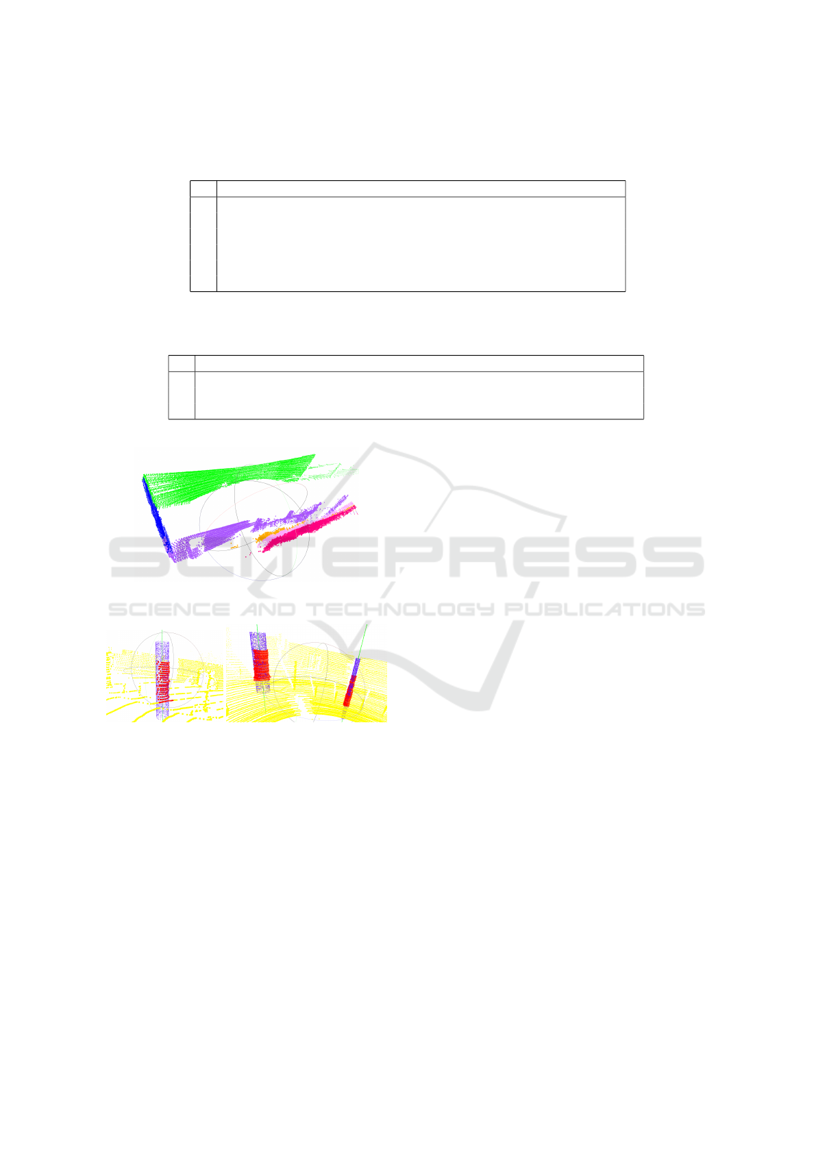
Table 3: Parameters of the detected planes in Figure 10. N denotes the number of points for which the plane ﬁtting is carried

out. Vectors P

and n denote a point of the plane, and the plane normal. Five out of the six plane are quasi parallel, the blue

one is perpendicular to the others.

color N P

1. green 31 743 (1.881, 0.999, -0.191) (-0.098, -0.995, 0,013)

2. magenta 10 328 (-2.486, 0.998, -1.071) (-0.059, -0.959, 0.055)

3. purple 9007 (-1.394, 0.996, 0.7974) (-0.235, -0.961, -0.148)

4. rose 4076 (-2.203, 0.989, -1.2377) (0.021, -0.940, 0.340)

5. blue 5698 (0.459, -0.041, 5.0901) (0.893, -0.449, 0.013)

6. orange 2428 (-2.086, 0.976, -0.572) (-0.143, 0.867, 0.478)

Table 4: Parameters of the detected cylinders in Figure 11. N denotes the number of the points of a cylinder. Vectors C and

W denote a point of the axis and the direction of the axis. r and h are the radius and the height value of the cylinder, ﬁnally,

E denotes the ﬁtting error given in Euclidean distance.

N C W r h E

1. 660 (5.560, 0.029, -0.432) (0.000,0.000, 1.000) 0.127 2.257 0.001

2. 782 (6.203, 7.609, -0.174) (-0.024,0.074, 0.996) 0.559 2.464 0.002

3. 263 (6.687, 16.955, 0.340) (0.000,0.078, 0.996) 0.487 2.352 0.006

Figure 10: Fitted planes of an outdoor test in case of high

noise because of mirroring.

Figure 11: Fitted cylinders of some outdoor measurements.

ACKNOWLEDGEMENTS

EFOP-3.6.3-VEKOP-16-2017-00001: Talent Man-

agement in Autonomous Vehicle Control Technolo-

gies – The Project is supported by the Hungarian

Government and co-ﬁnanced by the European Social

Fund.

REFERENCES

Awrangjeb, M. and Fraser, C. S. (2014). Automatic seg-

mentation of raw LIDAR data for extraction of build-

ing roofs. Remote Sensing, 6(5):3716–3751.

orck,

A. (1996). Numerical Methods for Least Squares

Problems. Siam.

Eberly, D. Fitting 3D Data with a Cylinder. http://

www.geometrictools.com/Documentation/Cylinder

Fitting.pdf. Online; accessed at 5th November 2018.

Eberly, D. Least Squares Fitting of Segments by Line or

Plane. https://www.geometrictools.com/Documentati

on/FitSegmentsByLineOrPlane.pdf. Online; accessed

at 5th November 2018.

Eberly, D. Least Squares Fitting on Data. http://www.geo

metrictools.com/Documentation/LeastSquaresFitt

ing.pdf. Online; accessed at 5th November 2018.

Fischler, M. and Bolles, R. (1981). RANdom SAmpling

Consensus: a paradigm for model ﬁtting with appli-

cation to image analysis and automated cartography.

Commun. Assoc. Comp. Mach., 24:358–367.

Grant, W. S., Voorhies, R., and Itti, L. (2013). Finding

planes in lidar point clouds for real-time registration.

In International Conference on Intelligent Robots and

Systems, pages 4347–4354.

Hartley, R. and Zisserman, A. (2003). Multiple view geom-

etry in computer vision. Cambridge University Press.

Nurunnabi, A. and andoderik Lindenbergh, Y. S. (2017).

Robust cylinder ﬁtting in three-dimensional point

cloud dara. In The International Archives of the Pho-

togrammetry, Remote Sensing and Spatial Informa-

tion Sciences, pages 63–70.

Pereira, M., Silva, D., Santos, V. M. F., and Dias, P. (2016).

Self calibration of multiple lidars and cameras on au-

tonomous vehicles. Robotics and Autonomous Sys-

tems, 83:326–337.

Pratt, V. (1987). Direct Least-squares Fitting of Algebraic

Surfaces. In Proceedings of the 14th Annual Con-

ference on Computer Graphics and Interactive Tech-

niques, SIGGRAPH ’87, pages 145–152.

Tsai, A., Hsu, C., Hong, I.-C., and Liu, W.-K. (2010). Plane

and boundary extraction from lidar data using cluster-

ing and convex hull projection. In IAPRS, pages 175–

179.

VISAPP 2019 - 14th International Conference on Computer Vision Theory and Applications

628

APPENDIX

Plane Fitting. The implicit form of a 3D plane is

usually given as



a b c d



x y z 1



= 0.

It can be written as P

X = X

P = 0 in short,

where P =



a b c d



and X =



x y z 1



con-

tain the plane parameters and the point coordinates

in homogeneous form. If the plane is represented

by a point P

and normal n, then the implicit form

is written as n



X − P



= 0, where

X =



x y z



The two plane representations are equivalent if

P =



−



and X =



X 1



Plane ﬁtting algorithms usually ﬁnd the plane that

is the closest one to the points. It can be carried out

by minimizing the algebraic error: if a point set {P

i = {1, 2, . . . , N} is given, the cost function to be min-

imized becomes

∑

i=1





This is equivalent to minimize the square of the

norm of the matrix-vector product AP:

, where

A =



. . . X



. It is well-known (Bj

orck,

1996) that the optimal solution for this problem is

that P is the eigenvector of matrix A

A corresponding

to the smallest eigenvalue if the length of the vector,

consisting of the plane parameters, is one: P

P = 1.

Sphere Fitting. We have tried several sphere ﬁtting

algorithms on LiDAR point clouds, it was found that

the method of (Eberly, c) is the most efﬁcient one for

this purpose, based on our experiences.

The equation of a general sphere is written

as (x − a)

+ (y − b)

+ (z − c)

= r

, where

C = [a b c]

is the center, and r the radius of the

sphere.

The sphere ﬁtting algorithm is based on min-

imizing squared error, where the error is deﬁned

as the difference between the estimated and real

distance from a surface point to the center of

the sphere: E(a, b, c, r) =

∑

i=1

− r)

,where l

− a)

+ (y

− b)

+ (z

− c)

is the length of the

radius to the i-th point (x

, y

, z

The partial derivates of E with respect to r, a, b

and c must be equal to zero at the minima. This leads

to the following equations:

a =

∑

i=1

∑

i=1

a − x

, b =

∑

i=1

∑

i=1

b − y

c =

∑

i=1

∑

i=1

c − z

, r =

∑

i=1

(2)

If one substitutes r into the last three equations,

the center coordinates of the sphere can be estimated

by ﬁxpoint-iteration. The offset value is the average

of the points. The four optimization steps are run one

after the other until convergence.

Cylinder Fitting. We suggest to apply the method

of (Eberly, a) for cylinder ﬁtting.

A cylinder can be represented by a point C of the

middle axis, and a direction, represented by unit vec-

tor W, of the axis, and radius r. Furthermore, it can be

deﬁned two more unit vectors U and V, which form in

conjunction with W a right-handed orthonormal co-

ordinate system. A surface point X of the cylinder

can be written as X = C + kU + uV + vW = C + RY,

where R =



U V W



is a rotation matrix and

Y =



k u v



contains the coordinates of the point in

the cylindric coordinate system.

When the distance between the axis and the sur-

face point X

is denoted by r

, similar to the sphere,

the error function becomes: E(r

, C, W) =

∑

i=1

−

)

,where r

= u

+ v

is the distance of the point to

the cylinder axis. The approximation of the radius is

the average of the estimated radius lengths from the

input surface points: r =

∑

i=1

The axis point can be calculated by an iteration,

where there is an offset value of the point, e.g. the

mean of the input points, and every iteration replace

the old value C for C + αU + βV. The α and β coef-

ﬁcients are obtained by the solution of the following

expression:

∑

i=1







∑

i=1



+ v



, (3)

which is an inhomogeneous system of linear equa-

tions. Althought the solution seems to depend on U

and V, it can be justiﬁed that the axis point can be

expressed with the X

input points and only the W

direction vector, because of U, V and W form an or-

thonormal system by deﬁnition. Hence, the direction

vector has to be approximated before the axis point.

The direction vector itself can be written by two

parameters θ

and θ

W = (cos θ

sinθ

, sin θ

sinθ

, cos θ

)

∈ [0,2π) θ

∈ [0,

] w

(θ

, θ

) ≥ 0.

(4)

An exhaustive search ﬁnds the optimal parameters

in our approach minimizing the cost function deﬁned

in Equation 4.

Robust Fitting of Geometric Primitives on LiDAR Data

629