
Using a Depth Heuristic for Light Field Volume Rendering
Se
´
an Martin, Se
´
an Bruton, David Ganter and Michael Manzke
School of Computer Science and Statistics, Trinity College Dublin, College Green, Dublin 2, Ireland
Keywords:
Light Fields, View Synthesis, Convolutional Neural Networks, Volume Rendering, Depth Estimation, Image
Warping, Angular Resolution Enhancement.
Abstract:
Existing approaches to light field view synthesis assume a unique depth in the scene. This assumption does not
hold for an alpha-blended volume rendering. We propose to use a depth heuristic to overcome this limitation
and synthesise views from one volume rendered sample view, which we demonstrate for an 8 × 8 grid. Our
approach is comprised of a number of stages. Firstly, during direct volume rendering of the sample view, a
depth heuristic is applied to estimate a per-pixel depth map. Secondly, this depth map is converted to a disparity
map using the known virtual camera parameters. Then, image warping is performed using this disparity map
to shift information from the reference view to novel views. Finally, these warped images are passed into a
Convolutional Neural Network to improve visual consistency of the synthesised views. We evaluate multiple
existing Convolutional Neural Network architectures for this purpose. Our application of depth heuristics is
a novel contribution to light field volume rendering, leading to high quality view synthesis which is further
improved by a Convolutional Neural Network.
1 INTRODUCTION
Light field technology is an exciting emergent subject,
allowing for extremely rich capture and display of vi-
sual information. Generating a light field from volu-
metric data produces significant perceptual enhance-
ments over directly volume rendering an image. For
example, medical practitioners could view the result
of Magnetic Resonance Imaging (MRI) scans in real-
time using a near-eye light field virtual reality device
(Lanman and Luebke, 2013) or The Looking Glass
(Frayne, 2018) without the drawback of current dis-
play devices, such as a single focal plane. These vi-
sualisations would allow for deeper understanding of
a patient’s anatomy before surgery and open new av-
enues for medical training. Although direct volume
rendering is possible in real-time for a single view-
point, this is infeasible with current technology for a
full light field due to the necessary increase in pixel
count. To bring the performance closer to interactive
rates, we propose a view synthesis method for light
field volume rendering by inferring pixel values using
a single sample image.
Recently, Convolutional Neural Networks
(CNNs) have been applied to view synthesis for
light fields of natural images, with the deep learning
approaches of (Wu et al., 2017) and (Kalantari
et al., 2016) constituting state of the art. (Srinivasan
et al., 2017) showed notable results using only one
image from a camera to synthesise an entire light
field. However, these methods are designed for
natural images which can reasonably be assumed
to have a well-defined depth. This is not the case
for volume rendering due to alpha compositing not
always resulting in an opaque surface. To increase
the suitability of these methods for volume rendering,
we present novel modifications.
Our proposed method synthesises a light field
from a single volume rendered sample image, which
we demonstrate for an 8 × 8 angular resolution light
field. We represent the light field as a structured grid
of images captured by a camera moving on a plane,
with the number of images referred to as the angu-
lar resolution. A depth heuristic is used to estimate
a depth map during volume ray casting, inspired by
the work of (Zellmann et al., 2012). This depth map
is converted to a disparity map using the known vir-
tual camera parameters. Image warping is performed
using the disparity map to shift information from the
single reference view to all novel view locations. Fi-
nally, the disparity map and warped images are passed
into a CNN to improve the visual consistency of the
synthesised views.
The results of this research show that the depth
heuristic applied during volume rendering produces
high quality image warping. Moreover, the CNN in-
134
Martin, S., Bruton, S., Ganter, D. and Manzke, M.
Using a Depth Heur istic for Light Field Volume Rendering.
DOI: 10.5220/0007574501340144
In Proceedings of the 14th Inter national Joint Conference on Computer Vision, Imaging and Computer Graphics Theory and Applications (VISIGRAPP 2019), pages 134-144
ISBN: 978-989-758-354-4
Copyright
c
2019 by SCITEPRESS – Science and Technology Publications, Lda. All rights reserved

creases the visual consistency of synthesised views,
especially for those views at a large distance from the
sample reference view, but the CNN must be retrained
for new volumes and transfer functions. Although
the presented method is not faster than directly vol-
ume rendering a light field, it is fast compared to ex-
isting light field angular resolution enhancement ap-
proaches. The bottleneck is the image warping proce-
dure, which takes 90% of the total time to synthesise
a light field, as opposed to our depth heuristic calcu-
lation or CNN. Our method is beneficial for complex
volumes because the time to synthesise a light field is
independent of the size and complexity of the volume
and rendering techniques.
2 RELATED WORK
Light Field View Synthesis. There are two pri-
mary paradigms for synthesising views for light fields
of natural images. One paradigm is to estimate some
form of geometry in the scene, commonly depth, and
base the view synthesis on this geometry. The other
paradigm focuses on the structure of light fields, using
expected properties of Epipolar-Plane Images (EPIs)
for view synthesis (Wu et al., 2017), or transforming
the problem to other domains with well-defined be-
haviour (Shi et al., 2014; Vagharshakyan et al., 2018).
These structure based approaches are slower than di-
rectly rendering the light field and are not applica-
ble to this problem. For instance, testing the state of
the art method by (Wu et al., 2017) was prohibitively
slow, taking 16 minutes to synthesise a full light field.
(Yoon et al., 2015) interpolated sets of light field
sub-aperture images with CNNs to produce a ×2 an-
gular resolution enhancement. This approach does
not take advantage of the light field structure and the
resulting resolution enhancement is too low to be use-
ful for volume rendering. Using a soft three dimen-
sional (3D) reconstruction (Penner and Zhang, 2017)
produces high quality view synthesis, but as we have
a 3D volume available, this route is not useful for us.
(Wanner and Goldluecke, 2014) formulate the view
synthesis problem as a continuous inverse problem,
but optimising the associated energy is too slow for
our needs.
Depth-based approaches are particularly relevant
to our problem, since we can estimate depth using vol-
umetric information. One such approach by (Kalan-
tari et al., 2016) uses deep learning to estimate depth
and colour, but they synthesise the light field view by
view. This leads to slow performance, taking roughly
12.3 seconds to generate a single novel view from
four input images of 541 × 376 resolution.
(Srinivasan et al., 2017) tackled the problem of
synthesising a four dimensional (4D) light field from
a single image. This problem is ill-posed because a
single image of a light field contains inadequate infor-
mation to reconstruct the full light field. The authors
alleviate this by using data-driven techniques trained
on images of objects from specific categories (e.g.
flowers) and by taking advantage of redundancies in
the light field structure. Their method accounts for
specular highlights, rather than assuming that all sur-
faces exhibit diffuse reflection. This is very relevant
for volume rendering, as surfaces are often anisotrop-
ically shaded. In contrast to most approaches, they
produce all novel views at once instead of synthesis-
ing each view separately. This is fast, synthesising a
187 × 270 × 8 × 8 light field in under one second on
a NVIDIA Titan X Graphics Processing Unit (GPU).
Because of the speed of this approach, the single in-
put view required, and the high quality results, our
approach follows a similar formulation.
To make the method of (Srinivasan et al., 2017)
more suitable for volume rendering, we propose to
use a depth heuristic during volume rendering as op-
posed to estimating depth for each ray in the light field
with a CNN. This will increase speed and account for
the transparent surfaces in volume rendering. Addi-
tionally, we propose to apply a two dimensional (2D)
CNN to improve the quality of the novel views instead
of their slower and potentially unnecessary 3D CNN.
CNN Architectures for 4D Light Fields. Al-
though we have volumetric information available,
CNNs using images from multiple views usually per-
form better than 3D CNNs on volumetric data because
current deep learning architectures are often unable
to fully exploit the power of 3D representations (Qi
et al., 2016). Due to limitations of 3D CNNs, (Wang
et al., 2016) demonstrate how to map a 4D light field
into a 2D VGG network (Simonyan and Zisserman,
2014) instead of using a 3D CNN. This is beneficial as
the weights of a pre-trained 2D model can be updated.
Additionally, although the 4D filters in 3D CNNs are
intuitive to use on a 4D light field, the number of pa-
rameters quickly explode. Since their paper is aimed
towards material recognition, we experiment with the
two most relevant methods for view synthesis to map
a 4D light field into a 2D CNN.
View Synthesis for Volume Rendering. Acceler-
ating volume rendering has long been an active re-
search area. Warping information from sample views
to synthesise new views (Mark et al., 1997; Mueller
et al., 1999; Lochmann et al., 2016) is feasible be-
cause rendered images do not tend to change dramat-
ically between viewpoints. Warping images is partic-
Using a Depth Heuristic for Light Field Volume Rendering
135
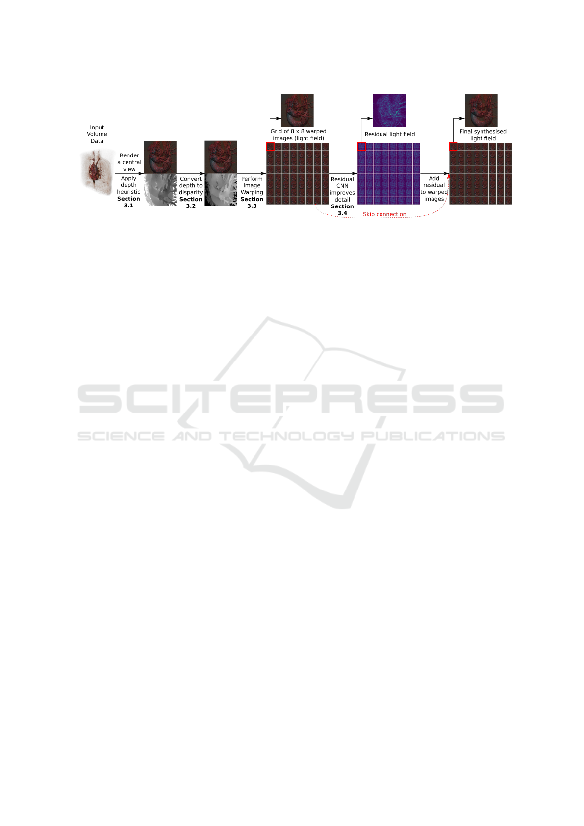
Figure 1: Our proposed light field synthesis method can be broken down into distinct stages, including an initial depth heuristic
calculation stage and a final CNN stage acting as a residual function to improve fine-grained detail.
ularly prevalent in remote rendering because a remote
machine with no GPU can warp an image produced
by a server until a new image is received. (Zellmann
et al., 2012) proposed to warp images received from
a remote server based on an additional depth chan-
nel. Due to alpha compositing resulting in transparent
surfaces with ill-defined depths, the authors present
multiple depth heuristics for image warping. They
found that modifying the ray tracer to return depth
at the voxel where the accumulated opacity along the
ray reaches 80% was the best balance between speed
and accuracy. We propose to apply an improved depth
heuristic to light field view synthesis for volume ren-
dering.
3 METHODOLOGY
Our goal is to synthesise a volume rendered light field
as a structured set of 8×8 novel views. The following
steps are involved in our light field synthesis (Figure
1).
1. Render a reference view by direct volume render-
ing and use a depth heuristic to estimate a depth
map during ray casting.
2. Convert the depth map to a disparity map using
the camera parameters.
3. Applying backward image warping to the refer-
ence view using the disparity map to approximate
a light field with an 8 × 8 angular resolution.
4. Apply a CNN to the warped images to improve
visual consistency. This is modelled as a residual
function which is added to the approximate light
field from the previous step.
We apply a CNN to help account for inaccuracies in
the depth map, specular highlights, and occlusions to
improve the visual coherency of synthesised views
over depth-based image warping.
3.1 Volume Depth Heuristics
Part of our contribution is applying depth heuristics
in volume rendering for light field angular resolu-
tion enhancement. Depth maps are useful for image
warping, but there is no unique depth for an alpha-
blended volume, so we apply a heuristic to determine
a per-pixel depth map. The depth of the first non-
transparent voxel along the ray is inaccurate as it tends
to be corrupted by highly transparent volume infor-
mation close to the camera. Using isosurfaces gives
a good view of depth, but these must be recalculated
during runtime if the volume changes. To produce a
more accurate depth map, we estimate a depth during
ray casting.
To produce a depth estimate, we improve upon
the best performing single pass depth heuristic from
(Zellmann et al., 2012). In their work, when a ray ac-
cumulates a fixed amount of opacity, the depth of the
current voxel is saved. However, this depth map is of-
ten missing information when a ray does not accumu-
late the desired opacity. To counteract this limitation,
we save a depth value when a ray accumulates a low
threshold opacity and overwrite that depth if the ray
later accumulates the high threshold opacity. This im-
proved the quality of the depth map and a comparison
of different depth heuristics is presented in Section
5.2.
3.2 Converting Depth to Disparity
We convert depth to disparity for image warping.
During rendering, a depth value from the Z-buffer
Z
b
∈ [0, 1] is converted to a pixel disparity value using
the intrinsic camera parameters as follows. The depth
buffer value Z
b
is converted into normalised device
co-ordinates, in the range [−1, 1], as Z
c
= 2 · Z
b
− 1.
Then, perspective projection is inverted to give depth
in eye space as
GRAPP 2019 - 14th International Conference on Computer Graphics Theory and Applications
136
Z
e
=
2 · Z
n
· Z
f
Z
n
+ Z
f
− Z
c
· (Z
f
− Z
n
)
(1)
Where Z
n
and Z
f
are the depths of the camera’s near
and far clipping planes in eye space, respectively.
Note that Z
n
should be set as close to the visualised
object as possible to improve depth buffer accuracy,
while Z
f
has negligible effect on the accuracy. Given
eye depth Z
e
, it is converted to a disparity value d
r
in
real units using similar triangles (Wanner et al., 2013)
as
d
r
=
B · f
Z
e
− ∆x (2)
Where B is the camera baseline, or distance between
two neighbouring cameras in the grid, f is the focal
length of the camera, and ∆x is the distance between
two neighbouring cameras’ principle points. Again,
using similar triangles, the disparity in real units is
converted to a disparity in pixels as
d
p
=
d
r
W
p
W
r
(3)
Where d
p
and d
r
denote the disparity in pixels and
real world units respectively, W
p
is the image width in
pixels, and W
r
is the image sensor width in real units.
If the image sensor width in real units is unknown, W
r
can be computed from the camera field of view θ and
focal length f as W
r
= 2 · f · tan(
θ
2
).
3.3 Disparity based Image Warping
Using the volume rendered reference view and esti-
mated disparity map, we warp the reference view to
63 novel positions in a grid. To synthesise a novel
view, a disparity map D : R
2
7→ R is used to relate
pixel locations in a novel view to those in the ref-
erence view. Let I : R
2
7→ R
3
denote a reference
Red Green Blue (RGB) colour image at grid position
(u
r
, v
r
) with an associated pixel valued disparity map
D. Then a synthesised novel view I
0
at grid position
(u
n
, v
n
) can be formulated as:
I
0
(x + d · (u
r
− u
n
), y + d · (v
r
− v
n
)) = I(x, y)
where d = D(x, y)
(4)
There are two paradigms for image warping with a
disparity map; forward mapping and backward map-
ping. Forward mapping is not surjective and maps
pixels from the reference view into the novel view,
which results in holes in the image, for example, in
occluded areas. Backward mapping works in the in-
verse direction. For each pixel in the novel view, the
most relevant information from the reference view is
assigned to that pixel. Therefore, it is surjective and
no holes are formed, but the reference view is usu-
ally oversampled. A comparison between backwards
mapping and forward mapping in terms of Peak Sig-
nal to Noise Ratio (PSNR) and Structural Similarity
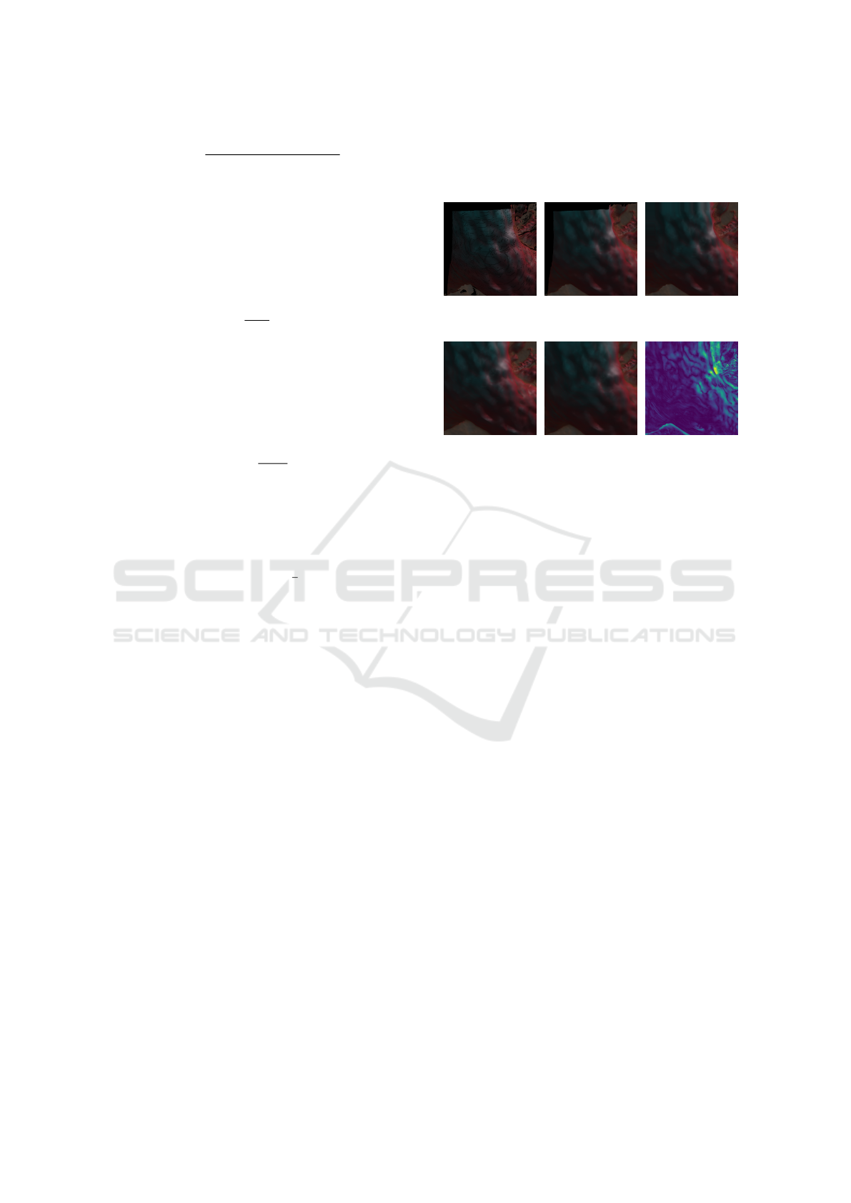
(SSIM) is presented in Figure 2.
(a) Forward warp
PSNR 22.81
SSIM 0.58
(b) Backward warp
PSNR 24.36
SSIM 0.79
(c) Stretching (b)
PSNR 27.92
SSIM 0.91
(d) Central
reference
(e) Ground truth
image
(f) Difference
between (c) and (e)
Figure 2: Demonstrating different warping methods to syn-
thesise the top left novel view at grid position (0, 0) from
the central reference view at position (4, 4) shown in Figure
(d). The forward warping in (a) has many cracks and holes.
Backward warping in (b) is smooth but is missing informa-
tion at the borders. As such, the border is stretched in (c),
which represents the final backward warping used.
For backward warping, pixels in the novel view
that should read data from a location that falls out-
side the border of the reference view were set to read
the closest border pixel in the reference view instead.
This would stretch the border of the reference view
in the novel view, rather than produce holes (Figure
2(c)).
3.4 Convolutional Neural Network
We apply a CNN to the grid of 64 images from the
previous step to improve the visual quality of the syn-
thesised light field. Giving the CNN access to all
warped images and the estimated disparity map al-
lows the network to learn to correct for errors at ob-
ject borders, modify the effect of specular highlights,
and predict information which is occluded in the ref-
erence view. This is achieved by framing the network
as a residual function that predicts only the correc-
tions needed to be made to the warped images to re-
duce the synthesis loss. The residual light field has
full range over the colour information, with values in
[−1, 1], to allow for removal of erroneous pixels and
addition of predicted data.
Because the light field is 4D, 3D CNNs which use
4D filters are intuitive to apply to this problem, but
using 2D convolutions leads to faster performance.
Using a Depth Heuristic for Light Field Volume Rendering
137
(Wang et al., 2016) demonstrated strong evidence that
3D CNNs can be effectively mapped into 2D archi-
tectures. To experiment with this, four primary net-
work architectures were implemented. Note that any
network’s Rectified Linear Unit activations have been
replaced by Exponential Linear Unit activations to be
consistent with the network from (Srinivasan et al.,
2017).
The first network tested was the 3D occlusion pre-
diction network from (Srinivasan et al., 2017), which
we will label Srinivasan3D. This network is struc-
tured as a residual network with 3 × 3 × 3 filters that
have access to every view. The input to Srinivasan3D
is all 64 warped images, and a colour mapped dispar-
ity map.
(He et al., 2016) introduced the concept of resid-
ual networks, which perform a series of residual func-
tions. The second network tested was a modified ver-
sion of ResNet18 (He et al., 2016), which we will call
StackedResNet. The input to StackedResNet is all
warped images and a colour mapped disparity map
which are stacked over the colour channels, a 195
channel input. To keep the spatial input dimensions
fixed, all spatial pooling is removed from ResNet18.
The first layer of ResNet18 is also replaced, as it is
intended to gather spatial information, and the input
is instead convolved into 64 features to gather angu-
lar information. The final fully connected layer of
ResNet18 is replaced by a convolutional layer with a
tanh activation function. Due to the removal of pool-
ing, pre-trained weights were not used for Stacke-
dResNet.
The third network, labelled StackedEDSR, was
based on the Enhanced Deep Super-Resolution
(EDSR) network of (Lim et al., 2017). EDSR is mod-
elled as a series of residual blocks which act upon a
single RGB image to learn relevant features before
performing spatial upsampling. The input to Stacked-
EDSR is the same as StackedResNet. As such, we
modify the first convolutional layer of EDSR to map
195 colour channels, instead of 3 colour channels,
to 256 features. StackedEDSR also removes the fi-
nal spatial upscaling performed by EDSR and applies
tanh activation after the last layer.
The final network, denoted AngularEDSR, is the
same network as EDSR, except for removal of spatial
upscaling at the last layer and application of tanh ac-
tivation at the final layer. To map the input into the
three colour channel input required for EDSR, angu-
lar remapping from (Wang et al., 2016) is applied to
create an RGB colour image. Consider a light field
sample with 8×8 images having 512×512 pixels and
three colour channels. This would be remapped into
an image having (8 · 512) × (8 · 512) pixels and three
colour channels. In this remapped image, the upper-
most 8 × 8 pixels would contain the upper-left pixel
from each of the original 8×8 views. The 3×3 filters
used in this architecture look at the nearest neighbours
to a view as opposed to all views as is the case for
the other networks tested. Pre-trained weights were
tested for both EDSR based networks, but they per-
formed poorly.
4 IMPLEMENTATION
Every experiment was performed on a computer with
16GB memory, an Intel i7-7700K @ 4.20GHz Cen-
tral Processing Unit (CPU), and a NVIDIA GeForce
GTX 1080 GPU running on Ubuntu 16.04. For deep
learning, the PyTorch library (Paszke et al., 2017),
version 0.40 was used with Cuda 9.1, cuDNN 7.1.2,
and NVIDIA driver version 390.30.
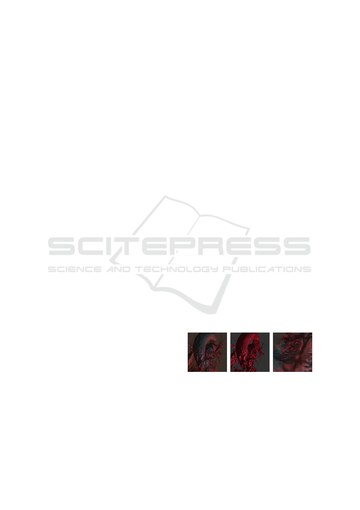
4.1 Data Collection
To demonstrate validity of the proposed method, an
MRI of a heart with visible aorta and arteries would
be used for training and validation. The heart volume
dataset has a resolution of 512×512×96 and is avail-
able online (Roettger, 2018b). See Figure 3 for exam-
ples of this dataset rendered. This volume was chosen
because the heart has a rough surface, and the aorta
and arteries create intricate structures which are dif-
ficult to reconstruct. See Figure 3(c) for an example
of a translucent structure in this dataset. The applied
transfer function does not contain high frequencies
which tend to reveal isosurfaces or geometry which
is static in texture because inaccurate depth maps can
still produce correct warping on large regions with a
static texture. Consequently, the depth map genera-
tion is well tested.
(a) Training
transfer function
(b) Simple
transfer function
(c) Translucent
structure
Figure 3: Demonstrating the training volume and transfer
function with images rendered in Inviwo.
Using Inviwo (Sund
´
en et al., 2015), a synthetic
light field dataset is captured. The light field captur-
ing geometry used is a “2D array of outward look-
ing (non-sheared) perspective views with fixed field
of view” (Levoy and Hanrahan, 1996). To capture the
GRAPP 2019 - 14th International Conference on Computer Graphics Theory and Applications
138
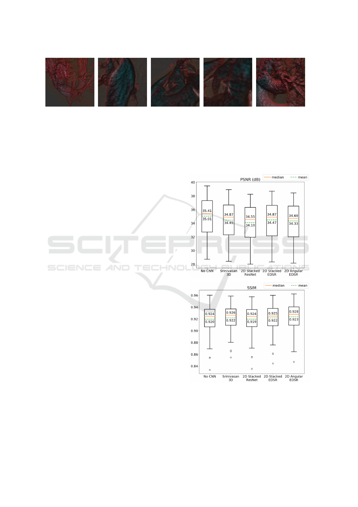
Figure 4: Sample training light field central sub-aperture views.
synthetic dataset, a Python script is created to move
the camera in Inviwo along a regular equidistant grid.
The cameras are shifted along the grid rather than ro-
tated to keep their optical axes parallel, removing the
need to rectify the images to a common plane. Each
light field sample has an angular resolution of 8 × 8,
with 512 × 512 spatial resolution. 2000 training light
fields are captured, and 100 separate validation light
fields. See Figure 4 for the central sub-aperture image
of five captured light fields.
Sampling was performed uniformly, rather than
focusing on particular sections of the heart. To in-
crease the diversity of the data captured, a plane with
a normal aligned with the camera view direction is
used to clip the volume for half the captured exam-
ples. This plane clipping can reveal detailed struc-
tures inside the volume and demonstrates the accu-
racy of the depth heuristic when the volume changes.
4.2 Training Procedure
To increase training speeds and the amount of avail-
able data, four random spatial patches of size 128 ×
128 are extracted from each light field at every train-
ing epoch. Additionally, training colour images have
a random gamma applied as data augmentation.
The CNNs are trained by minimising the per-pixel
mean squared error between the ground truth views
and the synthesised views. Network optimisation
was performed with Stochastic gradient descent and
Nesterov momentum. An initial learning rate of 0.1
was updated during learning by cosine annealing the
learning rate with warm restarts (Loshchilov and Hut-
ter, 2017). Gradients were clipped based on the norm
at a value of 0.4 and an L2 regularisation factor of
0.0001 was applied. Training takes about 14 hours us-
ing 2D CNN architectures with eight CPU cores used
for data loading and image warping.
5 EXPERIMENTS
5.1 Network Comparison for View
Synthesis
Figure 5: Comparing CNN architectures for view synthesis.
The box plots show PSNR and SSIM values averaged over
the 64 grid images for one hundred validation light fields.
The whiskers in the box plot indicate the data variability
and show the lowest datum and highest datum within 1.5 of
the interquartile range. The small circlular points outside of
the whiskers are outliers. The CNNs incur large loss at the
reference view position, especially for PSNR.
Using a Depth Heuristic for Light Field Volume Rendering
139
In Figure 5, the PSNR and SSIM metrics for each net-
work averaged over all light field sub-aperture images
are presented for the full validation set of one hun-
dred light fields. These experiments demonstrate that
the 3D convolutions performed in (Srinivasan et al.,
2017) can be effectively mapped into 2D CNNs as the
EDSR (Lim et al., 2017) based 2D networks outper-
form the slower 3D convolutions.
From Figure 5, it appears that none of the resid-
ual CNNs exhibit much performance difference from
geometrical warping. Investigating the results for
each synthesised sub-aperture view reveals further in-
sights. This is emphasised by the large loss in PSNR
and SSIM for the reference view position when using
a CNN. Warping does not change the reference view,
maintaining perfect PSNR of 100 and SSIM of 1.0.
However, when a residual CNN is applied it modi-
fies the reference view and this decreases to approxi-
mately 40 and 0.92 respectively. The reference view
could be used without adding the residual to it, but
this lessens the consistency of the resulting light field.
Figure 6 presents the difference in quality be-
tween image warping and the AngularEDSR CNN
per sub-aperture image location for one sample val-
idation light field. To summarise the results, images
far away from the central view exhibited lower loss
when a residual CNN was applied on top of image
warping. However, the CNN caused a degradation
in quality for central images. Additional evaluation
performed with the Learned Perceptual Image Patch
Similarity (LPIPS) metric (Zhang et al., 2018) using
the deep features of AlexNet (Krizhevsky et al., 2012)
to form a perceptual loss function agrees with the per
image values for SSIM and PSNR. See Figure 8 for
the bottom right sub-aperture view of this light field
from the validation set along with difference images
to visualise the effect of the CNN.
5.2 Depth Heuristic Comparison
To compare depth heuristics, ten light fields were cap-
tured without volume clipping. Five depth maps are
recorded:
1. OneDepth: The depth at 0.8 opacity during ray
casting.
2. TwoDepthFar: The depth at 0.8 opacity, and if
that is not reached, the depth at 0.3 opacity during
ray casting.
3. TwoDepthClose: The depth at 0.7 opacity, and
if that is not reached, the depth at 0.35 opacity
during ray casting.
4. IsoDepth: The depth of an isosurface at a value
of 80 which is precomputed on the CPU.
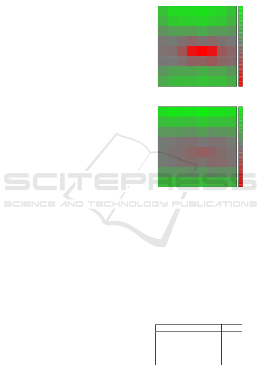
PSNR Difference
0.7 0.9 0.9 0.9 0.9 0.9 0.8 0.6
0.5 0.7 0.8 0.8 0.8 0.7 0.7 0.5
0.2 0.3 0.4 0.3 0.4 0.3 0.3 0.3
-0.0 0.0 -0.1 -0.2 -0.1 -0.1 -0.1 0.0
-0.1 -0.1 -0.3 -1.0 -1.2 -1.0 -0.3 -0.2
-0.0 0.0 -0.1 -0.2 -0.2 -0.3 -0.2 -0.1
0.3 0.4 0.4 0.4 0.5 0.4 0.4 0.3
0.4 0.6 0.6 0.6 0.7 0.6 0.6 0.5
1 2 3 4 5 6 7 8
Sub-Aperture Image x-index
1
2
3
4
5
6
7
8
Sub-Aperture Image y-index
-1
-0.5
0
0.5
1
SSIM Difference
0.012 0.013 0.013 0.013 0.014 0.013 0.013 0.012
0.008 0.009 0.008 0.008 0.009 0.008 0.008 0.008
0.004 0.004 0.003 0.003 0.004 0.003 0.003 0.004
0.000 -0.000 -0.001 -0.001 -0.000 -0.001 -0.001 0.001
0.000 -0.001 -0.001 -0.002 -0.003 -0.002 -0.001 -0.001
0.000 -0.000 -0.001 -0.001 -0.001 -0.002 -0.002 -0.001
0.003 0.003 0.003 0.002 0.003 0.002 0.003 0.003
0.007 0.008 0.007 0.007 0.008 0.007 0.007 0.007
1 2 3 4 5 6 7 8
Sub-Aperture Image x-index
1
2
3
4
5
6
7
8
Sub-Aperture Image y-index
-0.015
-0.01
-0.005
0
0.005
0.01
0.015
Figure 6: SSIM and PSNR difference after applying An-
gularEDSR to the warped images. Results are shown per
sub-aperture image location in an 8 ×8 grid. Position (5, 5)
is the location of the reference view and the loss in PSNR
at that position is scaled to make the graph more readable.
5. FirstDepth: The depth of the first non-transparent
voxel hit during ray casting.
Each of these depth maps is used to warp the cen-
tral light field sample image to all 64 grid locations.
The average PSNR and SSIM over the ten synthesised
light fields for each different depth map is presented
in Table 1. TwoDepthFar is the depth heuristic that
was selected for use in the training set, as it achieved
the highest SSIM in this experiment.
Table 1: Comparing quantitative results of image warping
with different depth maps averaged over 10 light fields.
Depth map type PSNR SSIM
OneDepth 34.63 0.907
TwoDepthFar 35.95 0.923
TwoDepthClose 35.97 0.922
IsoDepth 35.01 0.909
FirstDepth 27.96 0.802
GRAPP 2019 - 14th International Conference on Computer Graphics Theory and Applications
140
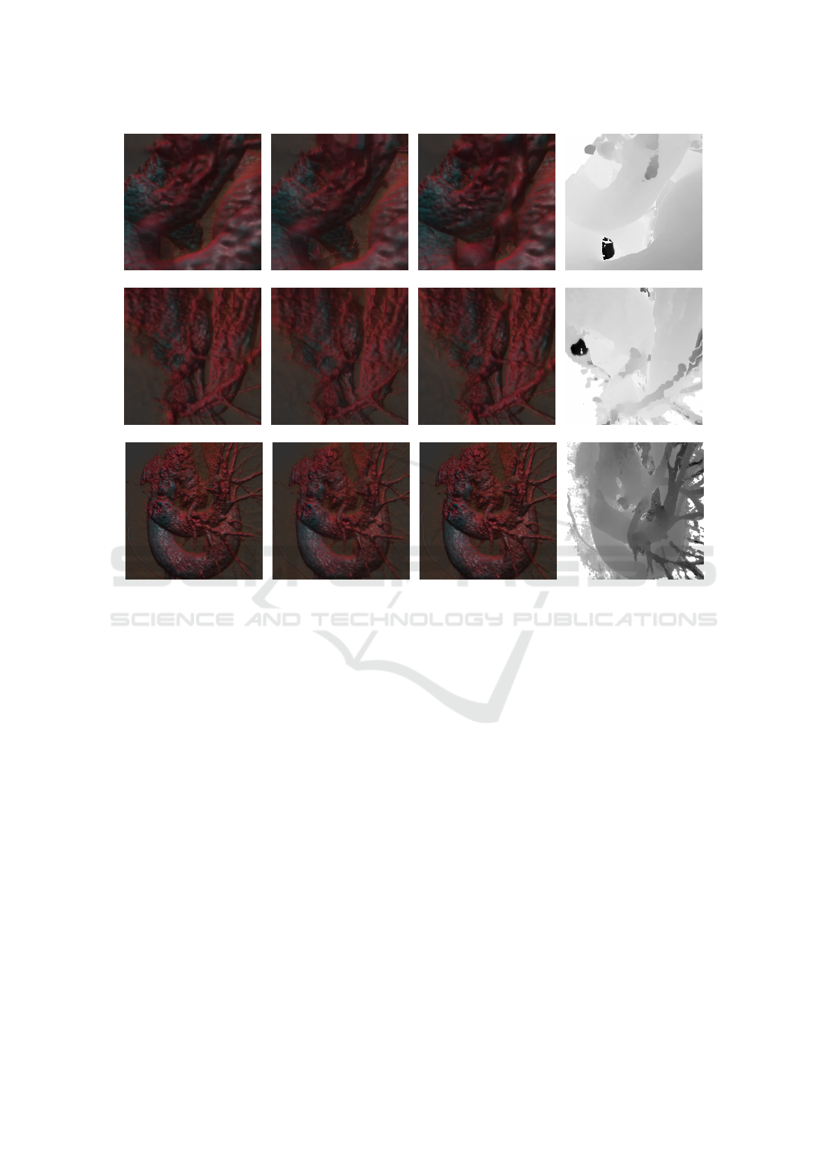
(a) Reference (b) Synthesised (c) Ground truth
(d) Disparity at (a)
(e) Reference (f) Synthesised (g) Ground truth
(h) Disparity at (e)
(i) Reference (j) Synthesised (k) Ground truth
(l) Disparity at (i)
Figure 7: Example synthesised upper-left images from the validation set. The first row has low performance due to the
translucent structure at the centre of the view. The second row has middling performance since the arteries are not perfectly
distinguished from the aorta. The third row has high performance with small inaccuracies, such as on the lower right edge of
the aorta. Disparity maps for the central reference views are presented in the final column.
5.3 Example Synthesised Light Fields
To investigate the method performance, an example
of a low, middling, and high quality synthesised light
field from the validation set is presented in Figure 7.
Figure 7(b) is a poor reconstruction due to the opaque
structure that should be present in the centre of the
view. This structure is not picked up by the dispar-
ity map, resulting in a large crack appearing in the
synthesised image. Figure 7(f) is a reasonably well
synthesised view. Most of the information is accu-
rately shifted from the reference view, but some arter-
ies lose their desired thickness and the image is not
very sharp. Figure 7(j) is an accurate synthesis. Some
errors are seen around object borders, such as on the
arch of the aorta, but overall it is hard to distinguish
from the ground truth information. Additional results
are presented in a supplementary video.
5.4 Time Performance in Inviwo
The presented method is currently not fast enough
for light field volume rendering at interactive rates.
On average, synthesising and displaying a light field
of 64 images with 512 × 512 pixels from the heart
MRI discussed in Section 4.1 takes 3.73 seconds in
Inviwo (Sund
´
en et al., 2015) if bilinear interpolation
is used for backward warping with the AngularEDSR
network. If nearest neighbours is used for warping in-
stead of bilinear interpolation the whole process takes
1.28 seconds, disregarding the time to pass informa-
tion through Inviwo. This is similar to the time taken
to directly render a light field in Inviwo, which takes
1.18 seconds.
The time for CNN view synthesis has far less de-
viation than directly volume rendering a light field,
because the latter depends heavily on the complex-
ity of the scene. A CNN performs the same oper-
ations regardless of input complexity, which results
Using a Depth Heuristic for Light Field Volume Rendering
141
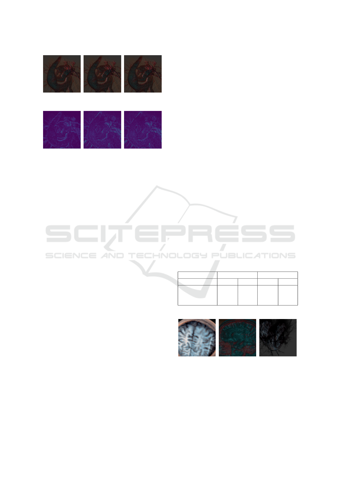
(a) AngularEDSR
PSNR 36.05
SSIM 0.909
(b) Warping alone
PSNR 35.59
SSIM 0.903
(c) Ground truth
PSNR 100.0
SSIM 1.000
(d) Difference
of (a) and (b)
(e) Difference
of (a) and (c)
(f) Difference
of (b) and (c)
Figure 8: The bottom right view in the light field which Fig-
ure 6 presents results for. Figure (d) visualises the residual
applied by the CNN to the warped images to improve visual
quality. The CNN detects broad edges to improve, such as
the central arch of the aorta, but fails to improve finer details
such as the arteries in the top right of the image.
in steady performance. Additionally, the CNN per-
formance is agnostic to the resolution of the volume
data and only depends on the spatial resolution of the
reference image. Accordingly, for very large com-
plex volumes with expensive rendering techniques,
this method could be applicable.
To understand the bottlenecks, we analyse the
breakdown of the 3.73 seconds to synthesise and dis-
play a light field in Inviwo with bilinear interpola-
tion. Rendering the reference view and passing in-
put and output information through Inviwo takes 0.91
seconds on average. Only 0.003 seconds is spent on
applying the depth heuristic, which is implemented
in the fragment shader. All CNNs tested complete
a forward pass in less than 0.2 seconds, with Angu-
larEDSR taking 0.047 seconds and Srinivasan3D tak-
ing 0.19 seconds. The time performance bottleneck is
image warping, which takes approximately 2.77 sec-
onds to warp a 512 × 512 image to a grid of 8 × 8
locations on the CPU. This is performed with bilin-
ear interpolation of pixel values. Using nearest neigh-
bours does not significantly jeopardise quality, and
takes 1.17 seconds. Although our image warping is
performed on the CPU due to GPU memory limita-
tions, the GPU based warping from (Srinivasan et al.,
2017) is also a performance bottleneck. For images of
size 192 × 192, their GPU accelerated warping takes
0.13 seconds, while our CPU warping with bilinear
interpolation takes 0.17 seconds.
Because of the time drawback, a 3D CNN which
directly took a reference view and associated depth
map to perform view synthesis was tested. This took
only 0.49 seconds on average, which is faster than di-
rect volume rendering. Despite this, the results were
low quality, averaging 26.1 PSNR and 0.83 SSIM.
The CNN learnt how to move information to new
views, but the colour consistency between views was
low. This method could be improved by a loss which
penalises a lack of colour consistency between views.
5.5 Performance on Unseen Data
Although the depth heuristic used during volume ren-
dering seems reasonable, there is no guarantee it
would perform well with different volumes and trans-
fer functions (TFs). Three experiments were per-
formed with the AngularEDSR architecture on ten
sample light fields in each case to test generalisation
of the depth heuristic. A new volume set of a head
MRI was used, available online (Roettger, 2018a)
with a different TF from the training set. Results are
presented in Table 2, and a central reference view for
each volume TF combination in Figure 9. The re-
sults show that the depth heuristic used and the im-
age warping applied using this generalise well. The
AngularEDSR network fails to generalise to unseen
volumes and transfer functions. This is hardly sur-
prisingly since the network has only ever seen one
volume and transfer function. As such, the CNN cur-
rently has to be retrained for new volumes or TFs, but
in future experiments we could attempt to generalise
this learning.
Table 2: Average results on transfer function and volume
combinations that are different from training.
Warping CNN
TF, volume PSNR SSIM PSNR SSIM
New TF, head 36.50 0.956 34.46 0.955
Seen TF, head 41.43 0.949 40.18 0.949
New TF, heart 37.78 0.932 36.89 0.927
(a) New volume
New TF
(b) New volume
Training TF
(c) Seen volume
New TF
Figure 9: Sample reference views used for synthesis of light
fields on unseen data.
GRAPP 2019 - 14th International Conference on Computer Graphics Theory and Applications
142

6 CONCLUSIONS AND FUTURE
WORK
Applying depth heuristics for the purposes of image
warping to synthesise views in light field volume ren-
dering produces good results and we recommend this
as a first step for this problem. Additionally, learning
a residual light field improves the visual consistency
of the geometrically based warping function, and is
useful for views far away from the reference view.
Our light field synthesis is fast compared to existing
methods but is still too slow to compete with direct
volume rendering in many cases. However, in con-
trast to light field volume rendering, the time for our
synthesis is independent of the volume resolution and
rendering effects and only depends on the resolution
of the sample volume rendered image.
Our view synthesis results for light field volume
rendering are of high quality and deep learning can
be effectively be applied to this problem, but the geo-
metrical image warping bottleneck prevents synthesis
at interactive rates.
In future work, we would be keen to consider
more datasets and transfer functions with various lev-
els of transparency to help generalise this approach.
We would also be interested in investigating further
image warping procedures to identify potential opti-
misations. A possible technique for effective synthe-
sis may be to use multiple depth heuristics and a CNN
to combine them into one depth map. Moreover, in-
corporating additional volume information alongside
a depth map and a volume rendered view could be
beneficial. Given the expense of 3D CNNs learning
over volumes, we expect that 2D CNNs learning from
multiple images are likely to dominate in future years
on volumetric data.
ACKNOWLEDGEMENTS
This research has been conducted with the financial
support of Science Foundation Ireland (SFI) under
Grant Number 13/IA/1895.
REFERENCES
Frayne, S. (2018). The looking glass. https:
//lookingglassfactory.com/. Accessed:
22/11/2018.
He, K., Zhang, X., Ren, S., and Sun, J. (2016). Deep resid-
ual learning for image recognition. In Proceedings of
the IEEE conference on computer vision and pattern
recognition, pages 770–778.
Kalantari, N. K., Wang, T.-C., and Ramamoorthi, R. (2016).
Learning-based view synthesis for light field cameras.
ACM Transactions on Graphics, 35(6):193:1–193:10.
Krizhevsky, A., Sutskever, I., and Hinton, G. E. (2012). Im-
agenet classification with deep convolutional neural
networks. In Advances in neural information process-
ing systems, pages 1097–1105.
Lanman, D. and Luebke, D. (2013). Near-eye light field
displays. ACM Transactions on Graphics (TOG),
32(6):220.
Levoy, M. and Hanrahan, P. (1996). Light Field Render-
ing. In Proceedings of the 23rd annual conference on
Computer graphics and interactive techniques, SIG-
GRAPH ’96, pages 31–42. ACM.
Lim, B., Son, S., Kim, H., Nah, S., and Lee, K. M. (2017).
Enhanced deep residual networks for single image
super-resolution. In The IEEE conference on com-
puter vision and pattern recognition (CVPR) work-
shops, volume 1, page 4.
Lochmann, G., Reinert, B., Buchacher, A., and Ritschel,
T. (2016). Real-time Novel-view Synthesis for Vol-
ume Rendering Using a Piecewise-analytic Represen-
tation. In Vision, Modeling and Visualization. The Eu-
rographics Association.
Loshchilov, I. and Hutter, F. (2017). SGDR: Stochastic
gradient descent with warm restarts. In International
Conference on Learning Representations.
Mark, W. R., McMillan, L., and Bishop, G. (1997). Post-
rendering 3d warping. In Proceedings of the 1997
symposium on Interactive 3D graphics, pages 7–16.
ACM.
Mueller, K., Shareef, N., Huang, J., and Crawfis, R. (1999).
Ibr-assisted volume rendering. In Proceedings of
IEEE Visualization, volume 99, pages 5–8. Citeseer.
Paszke, A., Gross, S., Chintala, S., Chanan, G., Yang, E.,
DeVito, Z., Lin, Z., Desmaison, A., Antiga, L., and
Lerer, A. (2017). Automatic differentiation in pytorch.
Penner, E. and Zhang, L. (2017). Soft 3d reconstruction
for view synthesis. ACM Transactions on Graphics,
36(6):235:1–235:11.
Qi, C. R., Su, H., Nießner, M., Dai, A., Yan, M., and
Guibas, L. J. (2016). Volumetric and multi-view cnns
for object classification on 3d data. In Proceedings of
the IEEE conference on computer vision and pattern
recognition, pages 5648–5656.
Roettger, S. (2018a). Head volume dataset.
http://schorsch.efi.fh-nuernberg.de/data/
volume/MRI-Head.pvm.sav. Accessed: 24/08/2018.
Roettger, S. (2018b). Heart volume dataset.
http://schorsch.efi.fh-nuernberg.de/
data/volume/Subclavia.pvm.sav. Accessed:
15/08/2018.
Shi, L., Hassanieh, H., Davis, A., Katabi, D., and Durand,
F. (2014). Light field reconstruction using sparsity in
the continuous fourier domain. ACM Transactions on
Graphics, 34(1):1–13.
Simonyan, K. and Zisserman, A. (2014). Very deep con-
volutional networks for large-scale image recognition.
arXiv preprint arXiv:1409.1556.
Srinivasan, P. P., Wang, T., Sreelal, A., Ramamoorthi, R.,
and Ng, R. (2017). Learning to sythesize a 4d rgbd
light field from a single image. In IEEE International
Using a Depth Heuristic for Light Field Volume Rendering
143

Conference on Computer Vision (ICCV), pages 2262–
2270.
Sund
´
en, E., Steneteg, P., Kottravel, S., Jonsson, D., En-
glund, R., Falk, M., and Ropinski, T. (2015). Inviwo -
an extensible, multi-purpose visualization framework.
In IEEE Scientific Visualization Conference (SciVis),
pages 163–164.
Vagharshakyan, S., Bregovic, R., and Gotchev, A. (2018).
Light field reconstruction using shearlet transform.
IEEE Transactions on Pattern Analysis and Machine
Intelligence, 40(1):133–147.
Wang, T.-C., Zhu, J.-Y., Hiroaki, E., Chandraker, M., Efros,
A. A., and Ramamoorthi, R. (2016). A 4d light-field
dataset and cnn architectures for material recognition.
In European Conference on Computer Vision, pages
121–138. Springer.
Wanner, S. and Goldluecke, B. (2014). Variational light
field analysis for disparity estimation and super-
resolution. IEEE Transactions on Pattern Analysis
and Machine Intelligence, 36(3):606–619.
Wanner, S., Meister, S., and Goldluecke, B. (2013).
Datasets and benchmarks for densely sampled 4d light
fields. In Vision, Modeling, and Visualization.
Wu, G., Zhao, M., Wang, L., Dai, Q., Chai, T., and Liu, Y.
(2017). Light field reconstruction using deep convo-
lutional network on epi. In IEEE Conference on Com-
puter Vision and Pattern Recognition (CVPR), pages
1638–1646.
Yoon, Y., Jeon, H.-G., Yoo, D., Lee, J.-Y., and So Kweon,
I. (2015). Learning a deep convolutional network for
light-field image super-resolution. In Proceedings of
the IEEE International Conference on Computer Vi-
sion Workshops, pages 24–32.
Zellmann, S., Aum
¨
uller, M., and Lang, U. (2012). Image-
based remote real-time volume rendering: Decoupling
rendering from view point updates. In ASME 2012
International Design Engineering Technical Confer-
ences and Computers and Information in Engineering
Conference, pages 1385–1394. ASME.
Zhang, R., Isola, P., Efros, A. A., Shechtman, E., and Wang,
O. (2018). The unreasonable effectiveness of deep
features as a perceptual metric. In Proceedings of
the IEEE Conference on Computer Vision and Pattern
Recognition (CVPR).
GRAPP 2019 - 14th International Conference on Computer Graphics Theory and Applications
144
