
Adaptive Method for Detecting Zero-Velocity Regions to Quantify
Stride-to-Stride Spatial Gait Parameters using Inertial Sensors
Mohamed Boutaayamou
1,2
, Cédric Schwartz
1
, Laura Joris
3
, Bénédicte Forthomme
1
, Vincent Denoël
1
,
Jean-Louis Croisier
1
, Jacques G. Verly
2
,
Gaëtan Garraux
4
and Olivier Brüls
1
1
Laboratory of Human Motion Analysis, University of Liège (ULiège), Liège, Belgium
2
INTELSIG Laboratory, Department of Electrical Engineering and Computer Science, ULiège, Liège, Belgium
3
Microsys Laboratory, Department of Electrical Engineering and Computer Science, ULiège, Liège, Belgium
4
GIGA - CRC In vivo Imaging, ULiège, Liège, Belgium
Keywords: Gait, Zero-Velocity Update, Algorithms, Concurrent Validation, Accuracy, Precision, Stride Length, Stride
Velocity, Gyroscope, Accelerometer, IMU.
Abstract: We present a new adaptive method that robustly detects zero-velocity regions to accurately and precisely
quantify (1) individual stride lengths (SLs), (2) individual stride velocities (SVs), (3) the average of SL, (4)
the average of SV, and (5) the cadence during slow, normal, and fast overground walking conditions in
young and healthy people. The measurements involved in the estimation of these spatial gait parameters are
obtained using only one inertial measurement unit attached on a regular shoe at the level of the heel. This
adaptive method reduced the integration drifts across consecutive strides and improved the accuracy and
precision in the spatial gait parameter estimation. The validation of the proposed algorithm has been carried
out using reference spatial gait parameters obtained from a kinematic reference system. The accuracy ±
precision results were for SLs: 0.0 ± 4.7 cm, −0.7 ± 4.4 cm, and −5.8 ± 5.8 cm, during slow, normal, and
fast walking conditions, respectively, corresponding to −0.1 ± 4.2 %, −0.5 ± 3.2 %, and −3.3 ± 3.0 % of the
respective mean SL. The accuracy ± precision results were for SVs: 0.0 ± 2.9 cm/s, −0.7 ± 3.8 cm/s, and
−6.7 ± 6.7 cm/s, during slow, normal, and fast walking conditions, respectively, corresponding to
−0.6 ± 3.3 %, −0.1 ± 4.5 %, and −3.5 ± 3.1 % of the respective mean SV. These validation results show a
good agreement between the proposed method and the reference, and demonstrate a fairly accurate and
precise estimation of these spatial gait parameters. The proposed method paves the way for an objective
quantification of spatial gait parameters in routine clinical practice.
1 INTRODUCTION
Stride length (SL) and stride velocity (SV) are gait
parameters of importance in multiple health-related
applications. For example, reduced gait speed in the
early stage of Parkinson’s disease is primarily related
to reduced SL (e.g., Morris et al., 1996; Hausdorff;
2009); SL estimation could thus help neurologists in
the early diagnosis of this disease. Conventional gait
analysis techniques, such as optoelectronic motion
capture systems, are often used as gold standards to
quantify such spatial gait parameters with high
accuracy (e.g., Woltring, et al., 1980; Schwartz et al.,
2015). Nevertheless, these systems are often
expensive and can only be used in a controlled
laboratory environment, which hinders their
widespread use. Besides, systems based on inertial
measurement units (IMUs) including miniaturized
inertial sensors such as accelerometers and
gyroscopes are becoming a reliable solution to handle
the extraction of relevant gait features outside the
laboratory environment (e.g., Aminian, et al. 2002;
Del Din et al., 2016; Song et al., 2018).
In this context, we have previously developed a
signal-processing algorithm to automatically extract
stride-to-stride temporal gait parameters and sub-
phase durations of a single stride. This algorithm was
based on accelerometer signals recorded at the level
of the heel and toe of the left/right foot during the
overground walking of young and healthy subjects
and older people (Boutaayamou et al., 2015;
Boutaayamou et al., 2018).
In this work, we extend this extraction algorithm
to include the estimation of spatial gait parameters,
Boutaayamou, M., Schwartz, C., Joris, L., Forthomme, B., Denoël, V., Croisier, J., Verly, J., Garraux, G. and Brüls, O.
Adaptive Method for Detecting Zero-Velocity Regions to Quantify Stride-to-Stride Spatial Gait Parameters using Inertial Sensors.
DOI: 10.5220/0007576002290236
In Proceedings of the 12th International Joint Conference on Biomedical Engineering Systems and Technologies (BIOSTEC 2019), pages 229-236
ISBN: 978-989-758-353-7
Copyright
c
2019 by SCITEPRESS – Science and Technology Publications, Lda. All r ights reserved
229

such as SL and SV. In order to minimize the
integration drifts across consecutive strides and to
improve the accuracy and precision in the estimation
of these spatial gait parameters, we present a new
adaptive method that robustly detects zero-velocity
update regions to further apply adequate initial
conditions in the integration of considered quantities.
In this work, we use this adaptive method to quantify
(1) individual SLs, (2) individual SVs, (3) the average
of SL, (4) the average of SV, and (5) the cadence
during slow, normal, and fast overground walking
conditions. The measurements involved in the
estimation of these spatial gait parameters are
obtained using only one IMU attached on a regular
shoe at the level of the heel. In addition, we consider a
concurrent, stride-to-stride, validation of the proposed
method/algorithm in young and healthy people. In this
validation, we compare the results to reference spatial
gait parameters (time-synchronously) provided by a
kinematic 3D system.
2 METHOD
2.1 Participants and Overground
Walking Setting
Three healthy young volunteers without any known
gait and lower limb pathology (one woman and two
men; mean (min–max) age = 26 years (24–27 years);
mean height = 1.79 m; mean weight = 74 kg)
participated in the walking experiments. Each of them
was equipped with a newly developed stand-alone
IMU-based hardware system. This system integrated
memory, microcontroller, battery, and four small
IMU modules (2 cm × 0.7 cm × 0.5 cm) including
three-axis gyroscopes (range: 2000 degree/second)
and three-axis accelerometers (range: ±16 g). This
IMU-based system can measure accelerations denoted
by
,
, and
, and angular velocity signals
denoted by
,
, and
along IMUs’ sensitive
axes as schematically illustrated in Figure 1.
The participants wore their own regular shoes.
Four IMUs were directly attached to the heel and toe
of each shoe. Gait data were synchronously recorded
at 200 Hz from these four IMUs. The participants
were also equipped with four active markers. Each
marker was attached on each IMU, i.e., the four
markers were also attached to the shoes at the level of
the heel and toe. A four-camera Codamotion system
(Charnwood Dynamics; UK) recorded gait data from
these active markers at 200 Hz. In this work, we
quantify SLs, SVs, and the cadence – for each foot –
from only the heel IMU measurements.
Before starting the measurements, volunteers took
sufficient time to get used to the instrumentation tools
and to the experimental procedure. During the tests,
they were asked to walk back and forth on a 10-meter
long track in a wide, clear, and straight hallway, at
their slow, normal, and fast speeds. Each participant
performed (in the following order) 5 slow, 5 normal,
and 5 fast walking tests. The total number of recorded
gait tests is then 45 tests. The duration of a single gait
test was 60 s. All of the walking tests were performed
at the Laboratory of Human Motion Analysis
(LAMH) of the University of Liège, Belgium.
Figure 1: The newly developed stand-alone IMU-based
hardware system is applied to left and right foot using four
three-axis IMUs. The schematic illustration shows the
position of the sensors, i.e., IMUs and the Codamotion
active markers. Two of these sensors are attached to each
shoe at the level of the heel and toe, respectively. The
proposed algorithm quantifies SLs and SVs – for each foot
– only from the heel IMU measurements.
2.2 Adaptive Method for Detecting
Zero-Velocity Update Regions
The proposed extraction algorithm relies on the
assumption of foot movements in sagittal plane. In
order to accurately and precisely quantify individual
SLs and SVs during overground slow, normal, and
fast walking, it is important to robustly detect zero-
velocity update regions to further determine suitable
initial conditions to be used in integration steps of
considered quantities. The principal originality of this
algorithm is the use of an adaptive method to robustly
detect these zero-velocity update regions without the
need of empirical threshold values.
To reduce the number of sensors, we consider
hereafter only heel IMU measurements in the sagittal
plane. For clarity, we consider only one foot for the
description of the algorithm. The algorithm would be
applied in the same way for the left and right foot.
BIOSIGNALS 2019 - 12th International Conference on Bio-inspired Systems and Signal Processing
230
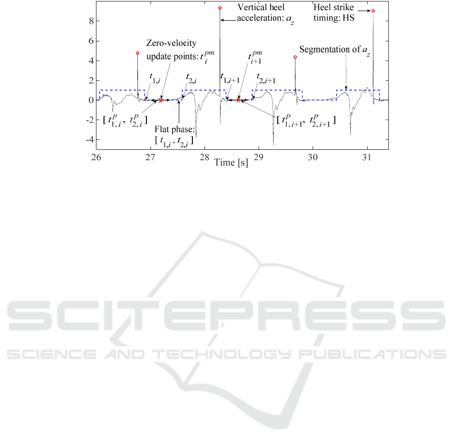
Figure 2: The proposed adaptive method is applied to the vertical heel acceleration and automatically detects set of points
that are candidates to be zero-velocity points where initial conditions are updated for each stride and for each partition .
All measured heel accelerations and angular
velocities are defined in the reference frame of the
heel IMU denoted by XYZ as illustrated in Figure 1.
We apply the proposed adaptive method to the
vertical heel acceleration signal to further estimate
SLs, SVs, and the cadence.
We first use our previously developed
segmentation method to parse heel acceleration data
into flat (motionless periods) and non-flat phases
(Boutaayamou et al., 2015). This segmentation
method has the advantage that it only determines
rough heel flat/non-flat phases and avoids to look
directly for specific gait events. Moreover, we
identify the heel strike (HS) timings adopting the
method from (Boutaayamou et al., 2015). We denote
time intervals corresponding to these flat phases by
[
,
,
,
] during each stride . Time intervals
,
,
,
refer to the zero-velocity update regions.
For each interval [
,
,
,
] having a length greater
than 20 samples, we consider partitions of
[
,
,
,
] into segments [
,
,
,
] of a length varying
from 10 samples to the length of [
,
,
,
], with an
overlap of 5 samples (see Figure 2). Given the
sampling frequency of 200 Hz, a sample
corresponds here to 5 milliseconds. For a given
partition , we calculate the variance of the vertical
heel acceleration signal in all associated segments
and determine the segment having the minimum
variance value, denoted by [
,
,
,
]. The midpoint
of [
,
,
,
] is denoted by
.
Considering a given
,
,
,
− having a length
greater than 20 samples − for stride , we emphasize
that we obtain a set of points
that are candidates
to be zero-velocity update points and not just one
zero-velocity update point as reported in the
literature (e.g., Mariani et al., 2010; Rebula et al.,
2013). Initial conditions are then updated at these
points
for each stride and for each partition .
For each interval [
,
,
,
] having a length strictly
less than 20 samples, we consider the midpoint of
[
,
,
,
] as a zero-velocity update point to be added
to the list of points
.
The extraction algorithm relies on successive
integrations in intervals [
,
]. For each stride
and for each partition , we estimate the inclination
of the foot in the sagittal plane,
, by integrating
the angular velocity in y-axis
(i.e., the yaw) in
the time interval [
,
]. The drift of this
integration is modeled as a straight line between
and
, and is subtracted from
to minimize this
drift and to ensure the initial conditions of this
integration:
=
,
and
=
,
.
Initial conditions
,
and
,
correspond to the
inclination of the foot during the flat phases
[
,
,
,
] and
,
,
,
, respectively. We use
the accelerometer as an inclinometer in these flat
phases to determine
,
as the mean value of
tan
(
/
) in [
,
,
,
], and
,
as the mean
value of tan
(
/
) in [
,
,
,
].
This is followed by a projection of the
acceleration on the horizontal axis of the lab
reference frame,
=a
cos
+a
sin
. We
obtain the horizontal velocity
by integrating
in
[
,
]. Again, the drift of this integration is
modeled as a straight line between
and
, and
is subtracted from
to minimize this drift and to
ensure the initial conditions of this integration:
=0 m/s and
=0 m/s for each
Ve
r
t
ical heel accele
r
a
t
ion [g]
Adaptive Method for Detecting Zero-Velocity Regions to Quantify Stride-to-Stride Spatial Gait Parameters using Inertial Sensors
231

Table 1: Mean and standard deviation (STD) of SLs, SVs, and cadence for each volunteer during slow (S), normal (N), and
fast (F) walking speed conditions with the associated mean, STD, minimum (Min) and maximum (Max) values of the flat
phase length (corresponding to the number of samples of 5 milliseconds).
SL (cm) SV (m/s) Cadence Flat phase length
Mean (STD) Mean (STD) Mean (STD) Min – Max
Volunteer 1
S 105.7 (8.3) 0.675 (0.069) 0.64 47 (10) 30 – 94
N 118.8 (7.4) 0.906 (0.054) 0.76
34 (10)
21 – 72
F 144.8 (7.2) 1.357 (0.078) 0.94
23 (6)
14 – 59
Volunteer 2
S 119.4 (7.1) 0.731 (0.045) 0.61 52 (9) 32 – 84
N 161.0 (7.1) 1.402 (0.073) 0.87
21 (7)
13 – 44
F 201.2 (7.7) 2.252 (0.103) 1.12
12 (2)
6 – 24
Volunteer 3
S 106.6 (11.7) 0.618 (0.138) 0.58 58 (19) 12 – 105
N 141.3 (5.2) 1.210 (0.069) 0.86
37 (6)
13 – 80
F 186.9 (7.9) 2.725 (0.188) 1.46
9 (2)
4 – 16
and . The horizontal position of the heel, , is
obtained by integrating
in [
,
], for each
and .
Finally, the stride length value of each stride ,
, is obtained by averaging all (
) found for .
For each stride , the stride velocity
is calculated
as
/(
−
). The average values of and
are thus estimated as the mean of
and
,
respectively. Moreover, the cadence is calculated as
the average of 1/(
−
); this average
corresponds to the average number of strides
performed during one second.
2.3 Concurrent Validation and
Evaluation Methods
We extracted reference spatial gait parameters from
the kinematic 3D Codamotion system to validate
concurrently, stride-to-stride, those extracted using
our algorithm, namely: (1) individual SLs, (2)
individual SVs, (3) the average of SL, (4) the
average of SV, and (5) the cadence.
Prior calculating these reference parameters, we
extracted reference HSs from measured heel
coordinates using the kinematic method reported in
(Boutaayamou et al., 2014). We extracted then
reference individual SLs from the horizontal heel
position signal. For each stride i, reference
individual SVs are determined as
/(
−
). Reference average values of and are
thus estimated as the mean of
and
,
respectively. Reference cadence is calculated as the
average of 1/(
−
).
We evaluated the level of agreement between
our method and the reference method in the
extraction of spatial gait parameters by quantifying
• The mean and standard deviation (STD) of
differences and relative differences,
• The mean and STD of absolute differences and
relative absolute differences,
• The root-mean-square (RMS) of differences and
relative differences,
for (1) individual SLs, (2) individual SVs, (3)
averages of SL, (4) averages of SV, and (5) the
cadence. The extraction accuracy and precision are
given by the mean and STD of differences,
respectively.
3 RESULTS
In this work, we focused on the results of gait tests
performed at speeds less than 11 km/h. We thus
excluded the last four fast walking tests of
volunteer 3 who walked at speeds ranging from
11.262 to 12.475 km/h.
A total of 551 gait cycles/strides – performed at
speeds less than 11 km/h – have been synchronously
recorded by both IMU-based system and reference
system. These strides have been obtained during
slow, normal, and fast walking conditions in young
and healthy volunteers with:
• Mean (STD) of SL = 110.8 cm (6.0 cm), mean
(STD) of SV = 0.675 m/s (0.051 m/s), and
cadence = 0.61 strides/s in slow walking
condition (n = 172 strides),
BIOSIGNALS 2019 - 12th International Conference on Bio-inspired Systems and Signal Processing
232

Table 2: Concurrent, stride-to-stride, validation results of the quantification of individual SLs and SVs, and averages of SL
and SV using our method (IMU) and the reference method (Ref) during slow (S), normal (N), fast (F) walking speed
conditions in young and healthy volunteers. These results are given as mean and standard deviation (STD) of differences
and relative differences, mean and STD of absolute differences (Abs) and relative absolute differences, and root-mean-
square (RMS) of differences and relative differences.
Individual SLs and SVs
(a)
Averages of SL and SV
(b)
Differences
(c)
:
SL (cm); SV(cm/s)
Relative
differences
(c)
(%)
Differences:
SL (cm); SV(cm/s)
Relative
differences (%)
Mean Abs RMS
(STD) (STD)
Mean
(STD)
Abs
(STD)
RMS Mean
(STD)
Abs
(STD)
RMS Mean
(STD)
Abs
(STD)
RMS
SL
S
0.0
(4.7)
3.7
(2.8)
4.6 −0.1
(4.2)
3.4
(2.6)
4.2 −0.1
(2.3)
1.9
(1.3)
2.2 −0.1
(2.0)
1.7
(1.1)
2.0
N
−0.7
(4.4)
3.5
(2.7)
4.4 −0.5
(3.2)
2.5
(2.1)
3.3 −0.7
(1.2)
1.0
(0.9)
1.3 −0.5
(0.8)
0.7
(0.6)
0.9
F
−5.8
(5.8)
6.8
(4.6)
8.2 −3.3
(3.0)
3.8
(2.3)
4.4 −5.6
(1.4)
5.6
(1.4)
5.8 −3.2
(0.9)
3.2
(0.9)
3.3
SV
S
0.0
(2.9)
2.3
(1.8)
2.9 −0.1
(4.5)
3.5
(2.8)
4.4 0.0
(1.3)
1.1
(0.7)
1.3 −0.1
(2.0)
1.6
(1.1)
1.9
N
−0.7
(3.8)
3.0
(2.4)
3.8 −0.6
(3.3)
2.6
(2.2)
3.4 −0.7
(0.9)
0.9
(0.7)
1.1 −0.6
(0.8)
0.7
(0.6)
0.9
F
−6.7
(6.7)
7.7
(5.4)
9.4 −3.5
(3.1)
4.0
(2.4)
4.7 −6.4
(1.8)
6.4
(1.8)
6.7 −3.4
(1.0)
3.4
(1.0)
3.5
(a)
Total number of individual strides = 551, with n=172, 193, and 186 strides, for S, N, and F, respectively.
(b)
Total number of gait tests = 41, with n=15, 15, and 11 averages, for S, N, and F, respectively.
(c)
The differences and relative differences are defined here as IMU−Ref and 100 × (IMU−Ref)/Ref, respectively.
Table 3: Results of the comparison between global average values (STD) of SL and SV, and the cadence obtained by our
IMU-based system and those obtained by the reference system.
IMU-based system Reference system Mean differences Mean relative absolute
differences (%)
SL (cm)
S 110.7 (7.4) 110.8 (6.0) −0.1 0.05
N 140.3 (17.9) 140.9 (17.7) −0.7 0.46
F 174.2 (29.0) 179.8 (29.2) −5.6 3.12
SV (m/s)
S 0.675 (0.061) 0.675 (0.051) 0.000 0.02
N 1.172 (0.213) 1.179 (0.212) −0.007 0.57
F 1.886 (0.533) 1.950 (0.543) −0.064 3.30
Cadence
(strides/s)
S 0.61 (0.04) 0.61 (0.04) −0.001 0.09
N 0.83 (0.05) 0.83 (0.05) −0.001 0.13
F 1.07 (0.16) 1.07 (0.16) −0.002 0.22
• Mean (STD) of SL = 140.9 cm (17.7 cm), mean
(STD) of SV = 1.179 cm/s (0.212 cm/s), and
cadence = 0.83 strides/s in normal walking
condition (n = 193 strides),
• Mean (STD) of SL = 179.8 cm (29.2 cm), mean
(STD) of SV = 1.950 cm/s (0.543 cm/s), and
cadence = 1.07 strides/s in fast walking
condition (n = 186 strides).
Table 1 provides spatial gait parameter values
for each volunteers, with the associated values of the
flat phase length during these three walking speed
Adaptive Method for Detecting Zero-Velocity Regions to Quantify Stride-to-Stride Spatial Gait Parameters using Inertial Sensors
233

conditions. A flat phase length corresponds to the
number of samples of 5 milliseconds.
Tables 2 shows the concurrent, stride-to-stride,
validation results of the extraction of individual SLs
and SVs during these three walking speed conditions.
These results correspond to the application of the
proposed adaptive zero-velocity update region
method to the vertical heel acceleration signal.
The accuracy (precision) of the extraction of
individual SLs was 0.0 cm (4.7 cm), −0.7 cm
(4.4 cm), and −5.8 cm (5.8 cm) during slow, normal,
and fats walking condition, respectively,
corresponding to −0.1 % (4.2 %), −0.5 % (3.2 %),
and −3.3 % (3.0 %) of the respective mean SL.
The accuracy (precision) of the extraction of
individual SVs was 0.0 cm/s (2.9 cm/s), −0.7 cm/s
(3.8 cm/s), and −6.7 cm/s (6.7 cm/s) during slow,
normal, and fats walking condition, respectively,
corresponding to −0.1 % (4.5 %), −0.6 % (3.3 %),
and −3.5 % (3.1 %) of the respective mean SV.
Moreover, individual SLs could be quantified
with a mean (STD) of absolute differences of 3.7 cm
(2.8 cm), 3.5 cm (2.7 cm), and 6.8 cm (4.6 cm) for
slow, normal, and fast walking conditions,
respectively, corresponding to 3.4 % (2.6 %), 2.5 %
(2.1 %), and 3.8 % (2.3 %) of the respective mean SL.
Individual SVs could be also quantified with a
mean (STD) of absolute differences of 2.3 cm/s
(1.8 cm/s), 3.0 cm/s (2.4 cm/s), and 7.7 cm/s
(5.4 cm/s) for slow, normal, and fast walking
conditions, respectively, corresponding to 3.5 %
(2.8 %), 2.6 % (2.2 %), and 4.0 % (2.4 %) of the
respective mean SV.
RMS differences between SLs quantified by both
MU-based system and reference system were 4.6 cm,
4.4 cm, and 8.2 cm for slow, normal, and fast walking
conditions, respectively, corresponding to 4.2 %,
3.3 %, and 4.4 % of the respective mean SL.
RMS differences between SVs quantified by
both MU-based system and reference system were
2.9 cm/s, 3.8 cm/s, and 9.4 cm/s for slow, normal,
and fast walking conditions, respectively,
corresponding to 4.4 %, 3.4 %, and 4.7 % of the
respective mean SV.
Table 2 provides also quantitative values of the
averages of SL and SV obtained for the 41 gait tests
including 15, 15, and 11 tests in slow, normal, and
fast walking conditions, respectively. As mentioned
above, we emphasize that we considered the results
of 11 fast walking tests instead of 15 ones since we
excluded four gait tests performed – by volunteer 3 –
at speeds greater than 11 km/h; such walking speeds
are not the focus of this work.
Tables 3 shows the validation results of the
quantification of global average values of SL and
SV, and the cadence during the three walking speed
conditions in young and healthy volunteers. We
quantified the average value of SL with a mean of
differences (mean of relative absolute differences) of
−0.1 cm (0.05 %), −0.7 cm (0.46 %), and −5.6 cm
(3.12 %) for slow, normal, and fast walking
conditions, respectively. We quantified also the
average value of SV with a mean of differences
(mean of relative absolute differences) of 0.000 m/s
(0.02 %), −0.007 m/s (0.57 %), and −0.064 m/s
(3.30 %) for slow, normal, and fast walking
conditions, respectively. In addition, we quantified
the cadence with a mean of differences (mean of
relative absolute differences) of −0.001 strides/s
(0.09 %), −
0.001 strides/s (0.13 %), and −0.002
strides/s (0.22 %) for slow, normal, and fast walking
conditions, respectively.
4 DISCUSSION
We have presented a new adaptive method that
robustly detects zero-velocity update regions for
accurately and precisely quantifying (1) individual
SLs, (2) individual SVs, (3) the average of SL, (4)
the average of SV, and (5) the cadence during slow,
normal, and fast overground walking conditions in
young and healthy people. Data involved in this
quantification are the measurements obtained with
only one IMU attached on a regular shoe at the level
of the heel. This adaptive method aimed to reduce
the integration drifts across consecutive strides and
to improve the accuracy and precision in the spatial
gait parameter estimation.
A concurrent, stride-to-stride, validation of the
proposed algorithm has been carried out using
reference spatial gait parameters obtained from a
kinematic reference system (used as gold standard).
The experimental results show a good agreement
between our algorithm and the reference, and
demonstrate a fairly accurate and precise
quantification of the spatial gait parameters.
The detection accuracy ± precision of individual
SLs using the present algorithm ranged from
−0.7 ± 4.4 cm to 0.0 ± 4.7 cm for walking speeds
ranging from 2.43 ± 0.25 km/h to 5.05 ± 0.26 km/h,
corresponding to a range of −0.5 ± 3.2 % to
−0.1 ± 4.2 % of the respective mean SL. Moreover,
we quantified individual SLs with an
accuracy ± precision of −5.8 ± 5.8 cm for walking
speeds ranging from 4.88 ± 0.28 km/h to
9.81 ± 0.68 km/h.
BIOSIGNALS 2019 - 12th International Conference on Bio-inspired Systems and Signal Processing
234

In addition, the detection accuracy± precision of
individual SVs using the present algorithm ranged
from −0.7 ± 3.8 cm/s to 0.0 ± 2.9 cm/s for walking
speeds ranging from 2.43 ± 0.25 km/h to
5.05 ± 0.26 km/h, corresponding to a range of
−0.6 ± 3.3 % to −0.1 ± 4.5 % of the respective mean
SV. Moreover, we quantified individual SVs with an
accuracy± precision of −6.7 ± 6.7 cm/s for walking
speeds ranging from 4.88 ± 0.28 km/h to
9.81 ± 0.68 km/h, corresponding to −3.5 ± 3.1 % of
the respective mean SV.
We compared theses obtained results to
previously published results for the estimation of SL
and SV during each walking speed condition in
young and healthy volunteers as follows:
• Slow walking speed: compared to RMS values
reported in (Song et al., 2018) (i.e., 8.2 cm for
SL, 5.9 cm/s for SV), the present method
improves these values by approximatively a
factor of 2 (i.e., 4.6 cm for SL, 2.9 cm/s for SV),
• Normal walking speed: compared to the results
reported in (Mariani et al., 2010) (i.e., 2.4 ± 7.5
cm (2.1 ± 6.8%) for SL; 2.2 ± 6.2 cm/s
(2.4 ± 6.1 %) for SV), in (Aminian et al., 2002)
(i.e., RMS = 7.cm (7.2%) for SL and
RMS = 6 cm/s (6.7 %) for SV), in (Rampp et al.,
2015), the accuracy, precision and RMS are
improved by the present method (i.e.,
−0.7 ± 4.4 cm (−0.5 ± 3.2%) and RMS = 4.4 cm
(3.3 %) for SL; −0.7 ± 3.8 cm/s (−0.6 ± 3.3 %)
and RMS = 3.8 cm/s (3.4 %) for SV).
• Fast walking speed: compared to RMS values
reported in (Song et al., 2018) (i.e., 21.4 cm for
SL and 12.9 cm/s for SV), the present method
improves these values (i.e., 8.2 cm for SL and
9.4 cm/s for SV).
Compared to commercial trunk accelerometer
systems (e.g., Auvinet et al., 1999), which only
provide global gait features, the proposed system
(hardware and algorithm) is capable to extract stride-
to-stride spatial gait parameters. The stride-to-stride
extraction may be a huge advantage in the gait
analysis of some specific population such as
Parkinson’s disease patients who experience
freezing of gait, a sudden and brief episodic
alteration of strides regulation.
We emphasize that the proposed IMU-based
hardware system can time-synchronously record
signals from up to four IMU sensors. The proposed
algorithm can thus quantify the left/right step length,
the symmetry, and the regularity of the spatial gait
parameters.
The proposed IMU-based system can measure
spatial gait parameters in a very large number of
strides without the need of controlled laboratory
conditions. We believe that this novel IMU-based
system offers perspectives for use in a routine
clinical practice to deal with abnormal gait (e.g., gait
of patients with Parkinson’s disease).
5 CONCLUSION
We presented a new adaptive method that robustly
detects zero-velocity regions for accurately and
precisely quantifying (1) individual SLs, (2)
individual SVs, (3) the average of SL, (4) the
average of SV, and (5) the cadence during slow,
normal, and fast overground walking conditions in
young and healthy people. This method reduces the
number of foot-mounted IMUs for estimating spatial
gait parameters. The advantages of this method can
be summarized as follows:
• Only two IMUs are required, i.e., one for each
shoe at the level of the heel. This contributes to a
simplification of the proposed wearable IMU-
based system, thus resulting in reducing the costs
and time needed to attach the system on the body.
• This method is concurrently validated for
consecutive strides during slow, normal, and fast
overground walking conditions. The validation
used reference spatial gait parameters provided
by a kinematic system (used as gold standard).
• Compared to previous studies, the proposed
method improves the accuracy, precision and
RMS of the estimation of SLs and SVs during
slow, normal, and fast overground walking
conditions in young and healthy people.
The proposed method paves the way for an
objective quantification of spatial gait parameters in
routine clinical practice. This opens new perspectives
for use in clinical contexts to deal with abnormal gait
(e.g., gait of patients with Parkinson’s disease).
ACKNOWLEDGEMENTS
We would like to thank F. Dupont, Ph. Laurent, and
all the team of the Microsys Laboratory of the
University of Liège (ULiège) for their help in the
development of the hardware part of the IMU-based
system used in the present work. We also would like
to thank P. Harmeling (ULiège) for his technical
assistance and Professor Ph. Vanderbemden (ULiège)
for allowing us to use his laboratory facilities.
Adaptive Method for Detecting Zero-Velocity Regions to Quantify Stride-to-Stride Spatial Gait Parameters using Inertial Sensors
235

REFERENCES
Aminian, K., Najafi, B., Leyvraz, P.F. et al. (2002).
Spatio-temporal parameters of gait measured by an
ambulatory system using miniature gyroscopes. J. of
Biomechanics, 35, 689-699.
Auvinet, B., Chaleil, D., and Barrey, E. (1999). Analyse
de la marche humaine dans la pratique hospitalière par
une méthode accélérométrique. Revue du Rhumatisme,
66(7–9) :447–457.
Boutaayamou, M., Schwartz, C., Denoël, V., et al (2014).
Development and validation of a 3D kinematic-based
method for determining gait events during overground
walking. In International Conference on 3D Imaging,
Liège, Belgium, 1–6.
Boutaayamou, M., Gillain, S., Schwartz, et al. (2018).
Validated assessment of gait sub-phase durations in
older adults using an accelerometer-based ambulatory
system. In Proc. of the 11
th
International Joint
Conference on Biomedical Engineering Systems and
Technologies, 4:248–255.
Boutaayamou, M., Schwartz, C., Stamatakis, J., et al.
(2015). Development and validation of an
accelerometer-based method for quantifying gait
events. Medical Engineering & Physics, 37:226–232.
Del Din, S., Godfrey, A., & Rochester, L. (2016).
Validation of an accelerometer to quantify a
comprehensive battery of gait characteristics in
healthy older adults and Parkinson's disease: toward
clinical and at home use. IEEE J. Biomedical and
Health Informatics, 20(3), 838-847.
Hausdorff, J.M. (2009). Gait dynamics in Parkinson’s
disease: common and distinct behavior among stride
length, gait variability, and fractal-like scaling. Chaos:
Chaos: An Interdisciplinary Journal of Nonlinear
Science, 19(2), 026113.
Mariani, B., Hoskovec, C., Rochat, S., et al. (2010). 3D
gait assessment in young and elderly subjects using
foot-worn inertial sensors. J. of biomechanics, 43(15),
2999-3006.
Morris, M.E., Iansek, R., Matyas, T.A., et al. (1996).
Stride length regulation in Parkinson's disease:
normalization strategies and underlying mechanisms.
Brain, 119(2), 551–568.
Rampp, A., Barth, J., Schülein, S., Gaßmann, K.-G.,
Klucken, J., and Eskofier, B. M. (2015). Inertial
sensor-based stride parameter calculation from gait
sequences in geriatric patients. IEEE Trans. on
Biomedical Engineering, 62(4):1089–1097.
Rebula, J.R., Ojeda, L.V., Adamczyk, P.G., et al. (2013).
Measurement of foot placement and its variability with
inertial sensors. Gait & Posture, 38(4):974–80.
Schwartz, C., Denoël, V., Forthomme, B., et al. (2015).
Merging multi-camera data to reduce motion analysis
instrumental errors using Kalman filters. Computer
Methods in Biomechanics and Biomedical
engineering, 18(9), 952-960.
Song, M., & Kim, J. (2018). An ambulatory gait
monitoring system with activity classification and gait
parameter calculation based on a single foot inertial
sensor. IEEE Trans. on Biomedical Engineering,
65(4), 885-893.
Woltring, H. J., & Marsolais, E. B. (1980). Optoelectric
(Selspot) gait measurement in two-and three-
dimensional space–A preliminary report. Bulletin of
Prosthetics Research, 10, 46-52.
BIOSIGNALS 2019 - 12th International Conference on Bio-inspired Systems and Signal Processing
236
