Probabilistic Method for Estimation of Spinning Reserves in

Multi-connected Power Systems with Bayesian Network-based

Rescheduling Algorithm

Yerzhigit Bapin

and Vasileios Zarikas

1,2

School of Engineering, Nazarbayev University, 56 Kabanbay Batyr ave., Astana, Kazakhstan

Department of Engineering Informatics, University of Thessaly, Greece

Keywords: Spinning Reserve, Interconnected Power Systems, Bayesian Network, Probabilistic Reserve Estimation,

Power System Reliability.

Abstract: This study proposes a new stochastic spinning reserve estimation model applicable to multi-connected energy

systems with reserve rescheduling algorithm based on Bayesian Networks. The general structure of the model

is developed based on the probabilistic reserve estimation model that considers random generator outages as

well as load and renewable energy forecast errors. The novelty of the present work concerns the additional

Bayesian layer which is linked to the general model. It conducts reserve rescheduling based on the actual net

demand realization and other reserve requirements. The results show that the proposed model improves

estimation of reserve requirements by reducing the total cost of the system associated with reserve schedule.

1 INTRODUCTION

Reduction of the greenhouse gas emissions is

considered as one of the main issues faced by modern

society. Global warming and deteriorating ecological

situation on the planet require drastic changes to the

energy production technologies. Undoubtedly,

renewable energy and smart grid technologies have

crucial impacts in this transformation. During the last

decade, the total installed capacity of renewable

energy in the world has increased from 1.058 TW to

2.012 TW (Whiteman et al., 2017). It is expected that

the overall share of renewable energy will reach 40%

by 2040 (IEA, 2017). Nevertheless, to successfully

reach the renewable energy targets, many challenging

tasks need to be overcome in the near future. Because

of highly stochastic nature of renewable power,

accommodating large amounts of renewable

generation requires to have flexible grid from the

technical and operational perspectives.

Smooth integration of renewable energy

sources into the market and grid infrastructure will

require reconsideration of conventional operating

practices. Especially, significant attention should be

paid to the operational reliability of power systems.

Currently, there are two major reliability assessment

approaches prevailing in the electric power industry,

namely deterministic and probabilistic. Under

deterministic approach the reliability criteria are set

such that the grid system would be capable of

withstanding the loss of a single unit (N-1), or even

simultaneous loss of several power generating units

(N-k). The power system reliability evaluation based

on pure deterministic approach does not consider

stochastic processes occurring in the grid; however,

most of the present-day reliability criteria are based

on deterministic techniques. One of the reasons for

the widespread of deterministic reliability evaluation

methods is their relative simplicity and the lower

requirements applied to its input data (Billinton and

Allan, 1996). On contrary, reliability assessment

based on probabilistic techniques are more

sophisticated and require detailed information about

system characteristics such as generator outage rates,

load and renewable forecast errors, etc. The

advantage of probabilistic methods, as compared with

deterministic ones, is the ability to capture system

uncertainties and evaluate the magnitudes and effects

of these uncertainties on the operation of power

systems (Morales et al., 2014). Consequently, in

probabilistic reliability assessment methods, the

events are treated based on the likelihood of their

occurrence and the degree of their severity (Grigsby,

2013).

840

Bapin, Y. and Zarikas, V.

Probabilistic Method for Estimation of Spinning Reserves in Multi-connected Power Systems with Bayesian Network-based Rescheduling Algorithm.

DOI: 10.5220/0007577308400849

In Proceedings of the 11th International Conference on Agents and Artiﬁcial Intelligence (ICAART 2019), pages 840-849

ISBN: 978-989-758-350-6

The interest in utilization of the power system

reliability assessment using probabilistic methods has

been increasing with the growth of stochastic power

generation. Various reserve estimation

methodologies considering stochastic generation

have been proposed in the last few years.

Consideration of stochastic events in most of these

methodologies is conducted in two distinct ways: one

way requires imposing an upper limit to reliability

metrics determining the loss of load or loss of energy

expectation; another way includes an economic

penalty into the objective function. Conventional

probabilistic reliability assessment methods are

generally based on analytical or Monte-Carlo (MC)

techniques. Application of Bayesian network theory

in probabilistic reliability assessment has its

advantages over conventional analytical or MC-based

probabilistic methods. Particularly, Bayesian

Networks (BNs) aim to model conditional

dependence of system components and states, which

in turn allows making inference on the events of the

interest (Zarikas and Tursynbek, 2017). The BN-

based power system reliability assessment models

provide powerful and mathematically sound

framework to analyse complex and stochastic

domains making them an effective decision-making

tool for the grid system operators.

Although, the implementation of BNs in power

system analysis is relatively new approach, several

valuable works have been published during the last

decades. In one of the earliest studies on BN-based

power system reliability assessment (Yu et al., 1999),

the authors proposed the BN model for reliability

assessment of multi-area power systems. In this

study, the BN representation of a grid system is

conducted via system components, such as, power

generating capacity, tie-line capacity, interconnected

capacity etc. The information provided by the system

components is used to determine the system state

variable – Loss of Load (LOL). Here, LOL serves as

a binary variable identifying the states when demand

exceeds available power. The overall reliability of a

power system is evaluated in terms of the Loss of

Load Probability (LOLP). The methodology was

applied to the Three-Area IEEE Reliability Test

System (RTS). The reported LOLP results show close

proximity with the analytical method. Somewhat

similar approach presented in the study by (Limin et

al., 2002). The study constructs the BN of a grid

system in two steps. First, the fault tree graph is

created for each node using bucket elimination

(Dechter, 1996). During the second step, the minimal

path set is determined by using the graph search

technique. The study by (Yongli et al, 2006) proposes

an approximate inference algorithm on BN for

reliability assessment of power systems by time-

sequence simulation. The system components are

modeled using two-state Markov model. The

methodology constructs the fault tree graph and

corresponding BN for a system of interest using the

bucket elimination method. In the study by (Ebrahimi

and Daemi, 2009) the authors present a novel BN-

based grid system reliability assessment method. The

methodology uses the MC-based data sampling

technique to generate training data. The training data

is used to construct BN representing the power

system of interest. The methodology assesses the

reliability level of a system in terms of LOLP. The

methodology has been tested on the IEEE RTS. The

reported LOLP results are very close to those

obtained using conventional probabilistic techniques.

The main contribution of this paper is to present a

hybrid method for estimation of optimal amount of

spinning reserves in multi-connected power systems

using traditional probabilistic cost-benefit analysis in

conjunction with the BN-based reserve rescheduling

algorithm.

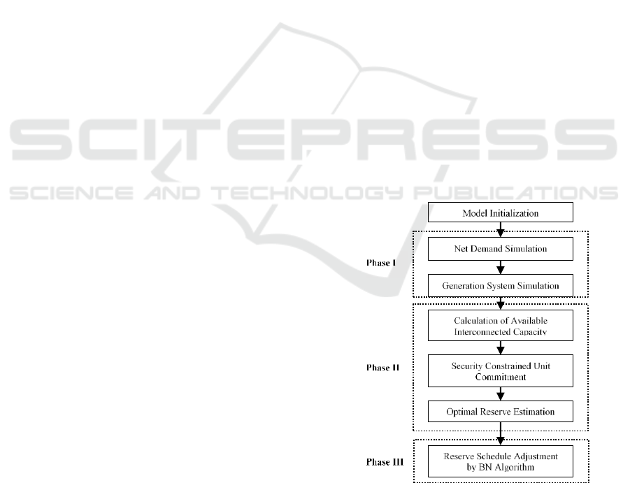
2 METHODOLOGY

The proposed methodology is carried out in three

phases. The flowchart of the proposed methodology

is presented in figure 1.

Figure 1: Flowchart of proposed model.

During the first phase, the reliability of the power

system of interest is evaluated neglecting its

interconnection with neighbouring systems. At the

Probabilistic Method for Estimation of Spinning Reserves in Multi-connected Power Systems with Bayesian Network-based Rescheduling

Algorithm

841

second phase, the Capacity Outage Probability Tables

(COPT) of the assisting power systems are obtained

using recursive algorithm and incorporated into

COPT of the assisted system. The reliability

evaluation is performed in terms of the Expected

Energy Not Supplied (EENS), which serves as a

metric for potential shortfall in supply of electricity to

consumers. As a result, the required amount of

spinning reserves is calculated based on the level of

reliability of the system and the capacity that is

available at a given time-period. At the final phase,

the BN-based algorithm is used to adjust the reserve

schedules based on the intra-hour actual data. The

detailed description of calculations conducted during

the first, second and third phases are described below.

2.1 Phase I

2.1.1 Net Demand Model

The proposed methodology considers renewable

power as negative load, and the net demand is defined

as the difference between load and renewable power

generation given by:

t t t

D L R

(1)

where D

is the net demand at period t, L

and R

are

the actual load and renewable energy production at

time period t. The forecast uncertainty is taken into

consideration by implementation of parametric

assumptions. Namely, the forecast error distribution

at time period t is given by:

~ ( ; )

Y F y



(2)

where Y

is the forecast error at time period t, F is the

distribution function of forecast error, y and



is the

set of parameters characterizing F (Morales et al.,

2014).

It should be noted that throughout this paper the

superscript t denotes the time periods and subscripts

i, j, l and k denote the power generating units,

interconnected reserve units, power transmission

lines and energy system areas respectively.

In this study, we assume that the load and

renewable forecast errors follow Normal distribution

with zero mean and the standard deviation given by

the following formulas (Ortega-Vazquez and

Kirschen, 2009):

Standard deviation of load forecast error:

100





(3)

where 





is the standard deviation of the load forecast

error distribution, k is a function depending on the

accuracy of the forecasting software and the

forecasted load at time period t.

Standard deviation of renewable forecast error:

5 50

R F I





(4)

where 





is the standard deviation of renewable

power forecast error distribution at time period t, 





is the forecasted renewable power at period t and 



is the total installed capacity of renewable power. The

former term stays constant throughout the simulation

horizon.

Figure 2: Seven-interval approximation of normal

distribution.

Discretization of load and renewable forecast

uncertainty can be done using seven-interval

approximation technique described in (Billinton and

Allan, 1996). Discretization is performed by dividing

the probability distribution of an error into an odd

number of equal intervals (Figure 2). These intervals

are considered as scenarios with individual

probabilities corresponding to the mid-point of each

interval. The lack of correlation between these errors

allows to calculate the net demand forecast error by

summation of the load and renewable forecast errors.

2.1.2 Generation System Model

The random outages of conventional units are

considered in the same fashion as it was done in

(Bapin et al., 2018). A random unavailability of

generating capacity can be modelled by representing

it as a Markov process. The availability and

unavailability of each generating unit in this case are

given by (5) and (6) (Billinton and Allan, 1996):

()

( ) ( )

up time

down time up time









(5)

UA

(6)

where 





and 





represent availability and

unavailability of unit i at time period t. Equations (5)

ICAART 2019 - 11th International Conference on Agents and Artiﬁcial Intelligence

842

and (6) represent the probability of finding the unit

either available or on forced outage at a given period

and can be used to create the Capacity Outage

Probability Table (COPT). Creation of COPT is

carried out using the recursive algorithm described in

(Billinton and Allan, 1996) and includes information

on available capacity and corresponding probabilities

for each system state. It should be noted that

throughout this paper the units’ capacity and power

production are denoted by capital P, whereas

lowercase p denotes probability.

The Expected Energy Not Supplied (EENS) due

to a random capacity outage m at time period t is

given by (Billinton and Allan, 1996):

[( ) ]

M S I

t t t

smm

EENS D P q q

  



  





  

(7)

where s is an index representing the net demand

scenario, 





is the available power when generation

system is at state m during time period t, q

and q

are

the probability of scenario of the net demand and

generating system availability respectively. Finally, I,

M and S are the total number of generating units,

generation system states and net demand scenarios

respectively. It is worth noting that, although variable







highly depends on the level of capacity

forced out of service, the probability of this outage

may have even stronger impact on the loss of energy

expectation. For instance, a simultaneous failure of

two or more units may cause significant disruption of

electricity supply. However, the probability of this

event is very low, thus the overall loss of energy

expectation would be lower as compared to the single

unit outage event.

2.2 Phase II

2.2.1 Interconnected Capacity

It is very common for an electric grid to have

interconnection with neighbouring systems, as most

of the time grid interconnections improve reliability

of the system and reduce its needs in reserve capacity

(Watchorn, 1950). The cross-border electricity

trading between interconnected systems is often done

based on the contractual agreements, where the

system operators define trading time, limits, ramp

rates etc. To account for interconnected capacity, the

proposed model utilizes the equivalent assisting unit

method as described in (Billinton and Allan, 1996).

The maximum assistance level provided by

interconnected system at time period t is given by the

minimum of available interconnected capacity and

tie-line capacity (Allan et al., 1986):

max , max

, , , ,

min ( ),

t inst t t

k j k j k j k l k

IR IR IR e IR r B







  









(8)

Where 





is the installed capacity of

interconnected unit j located in the assisting system k,







is the capacity committed for energy

generation of interconnected unit j located at assisting

system k during time period t, 





is the capacity

of interconnected unit j committed for provision of

spinning reserve at assisting system k during time

period t and 





is the maximum transmission

capacity of transmission line l. Finally, J and L are the

total number of interconnected reserve units and

transmission lines respectively. The maximum

capacity assistance level can be utilized to create a

capacity model in the same way as it was described in

the previous subsection. The resulting COPT is

regarded as an equivalent multi-stage generator,

which can be integrated in the existing capacity

model of an assisted system. During this phase, the

capacity assistance states are determined individually

for all assisting systems and added to the COPT of the

system of interest. It should be noted that in this paper

we assume that the interconnected capacity can only

participate in ancillary service market, thus it can only

provide up-spinning reserve service.

2.2.2 Stochastic Security Constrained Unit

Commitment

Objective Function.

In this study, the unit commitment problem is

expressed as a two-stage stochastic MILP. The first

stage involves conventional unit commitment with

stochastic reliability criteria to find the most optimal

energy production schedule. This stage is performed

for the base case scenario. The base case implies no

unit outage and results in the most economically

efficient unit commitment. The first-stage

optimization objective is to minimize the total cost of

system operation, where the total system operation

cost is given by:

Probabilistic Method for Estimation of Spinning Reserves in Multi-connected Power Systems with Bayesian Network-based Rescheduling

Algorithm

843

1 1 1

()

t t t

total i i i i

t t t t

i i i i

K J M

t t t

j k j k m

k j m

up up dw dw

C C P u CS

C R C R

CIR IR SC





  























 

(9)

where 



is the cost of power of generating unit i, 





is the power produced by unit i during time period t,







is the binary indicator of the status of generating

unit i at time period t (0 – not operating, 1 –

operating), 





is the start-up cost of unit i during

time period t, 





is the cost of power of unit i,

during time period t for providing the up-spinning

reserve, 





is the up-spinning reserve service

provided by unit i during time period t, 





is the

cost of power of unit i, during time period t for

providing the down-spinning reserve, 





is the

down-spinning reserve service provided by unit i

during time period t, 





is the cost of power

provided by interconnected unit j, located at energy

system k, during time period t, 





is the amount of

reserve provided by the interconnected unit j, located

at energy system k, during time period t. 





related to the second-stage decisions and is given by:



, , ,

t t t

m i i m

j k j m k

SC q C R

CIR IR

VOLL CE

















(10)

where 





is the cost of providing the spinning reserve

by intra-zonal unit i during time period t, 





is the

reserve service provided by intra-zonal unit i, at

system state m, during time period t, 





is the

amount of reserve provided by the interconnected unit

j, located at energy system k, at system state m, during

time period t. VOLL represents the value of lost load

– the financial loss of consumers due to interruption

in electricity supply, 





is the amount of curtailed

energy when generation system is in state m, during

time period t. The objective of the second-stage is to

find the most optimal reserve schedule by comparing

different scenarios.

First-Stage Constraints.

The objective function (9) must be minimized subject

to the set of constraints specified below. Note that to

reduce the computational burden and simplify the

model, the transmission line constraints are neglected

in this study. The equality between supply and

demand of electric power is specified by the power

balance constraint, which for all time instances is

given by:

()

t t t t t t t

i i i i i i

КJ

j k j k

кj

up dwD P u R u R u

IR u





  







(11)

In addition to equation (11) the conventional units are

subject to their operating constraints, such as

minimum up and down time, ramping and capacity

limits.

Second-Stage Constraints.

The second-stage constraints specifying all capacity

outage states is presented below. For all time periods

and scenarios, the power balance equation is given

by:

, , ,

1 1 1

()

t t t

m i i m i m

K J S

t t t

j k m s s m

k j s

up dwq P R R

IR D CE



  



  



 

(12)

Under this formulation of probabilistic reliability

criteria, the optimal spinning reserve requirement is

determined by counterweighting costs required to

operate the reserves with socioeconomic costs of

possible load curtailment. Reduction of spinning

reserves will negatively affect reliability of a system,

yet this reduction will be justified if the probability of

capacity outage is insignificant, or the social value of

curtailed load is very low.

2.3 Phase III

During recent years, rapid rise in computational

efficiency triggered the introduction of complex

machine learning algorithms into many different

areas. The scope of application of these algorithms

ranges from intellectual games, such as chess (David

et al., 2014) or go (van den Werf et al., 2003), medical

research (Eleftheriadou et al., 2009), (Deltsidou et al.,

2017), (Zarikas et al., 2015) to the power system

operation (Calabria et al., 2015) and (Steels and

Hanappe, 2008).

Aside from other machine learning algorithms,

BN-based algorithms have gained wide popularity

among power system and electrical engineers.

According to (Craciun et al., 2017) the application of

ICAART 2019 - 11th International Conference on Agents and Artiﬁcial Intelligence

844

BNs by the power system engineering researchers

include, but not limited to load forecasting, power

system reliability assessment and stability analysis,

electrical networks fault analysis and power system

state estimation.

Generally speaking, BN is a probabilistic

graphical model representing variables, their mutual

dependencies and associated probabilities (Zarikas,

2007). BN models are usually expressed in terms of

causal directed acrylic graphs (Jensen and Nielsen,

2011), where each variable has one or several directed

links with other variables. The objective of BN

models is to determine posterior conditional

probability distribution of an event in question based

on new evidence (Pearl, 2005). Equation (13)

represents the Bayes’ rule serving as the foundation

for BNs.

( | ) ( )

( | )

()

p B A p A

p A B



(13)

In this study, we propose a BN-based reserve

rescheduling algorithm. The main purpose of this

algorithm is to adjust the spinning reserve schedule

that was calculated during the first and second phases

of this methodology. The algorithm adjusts the

reserve requirement of the next closest time period

(t+1) based on the evidence received from the past

closest time period (t-1). Other parameters considered

by the algorithm during the adjustment procedure are

hour type (peak, non-peak) and day type (weekday,

weekend, holiday). The node specific properties, such

as, conditional probabilities or reserve

increase/decrease levels were set based on existing

practice, nevertheless, these properties can be easily

adjusted according to the user-specific preferences.

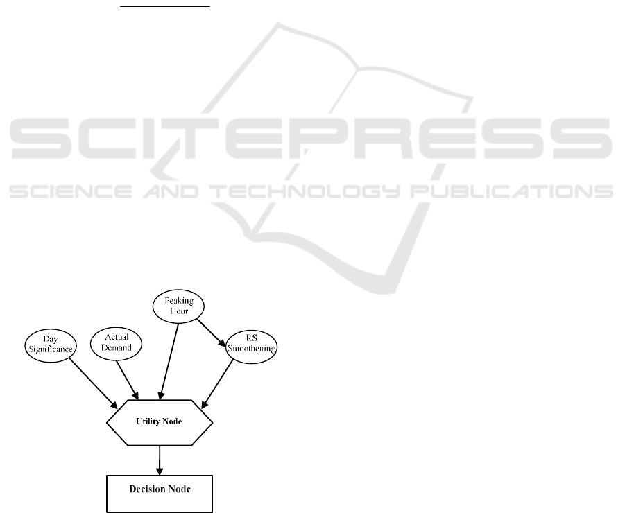
Figure 3: Part of the Influence Diagram of Proposed

Algorithm.

The algorithm was implemented in BayesiaLab 7

(Bayesia S.A.A., 2018). Figure 3 shows a simplistic

view of the decision influence diagram of the

proposed algorithm. The implemented BN consists of

2 such graphs each of every hour of one day.

The diagram consists of probabilistic, utility and

decision nodes each represented by elliptical,

hexagonal and rectangular-shaped figures

respectively. The detailed description of nodes is

provided below.

Probabilistic Nodes.

The probabilistic nodes denote variables specified

below:

Peaking Hour – denotes the variable containing

information about hour type and affects RS

Smoothening and Utility nodes. Usually, during peak-

hours energy systems pass through tremendous stress,

so the risk of electricity supply interruption is very

high. One way of reducing the level of this risk is to

increase the level of spinning reserve capacity. In

this model, the spinning reserve schedule adjustment

is set, such that, the reserve requirement is increased

by 10% for peaking time. The off-peak hours do not

affect previously calculated reserve schedule.

Day Significance – denotes the variable

containing information about day types and their

influence on spinning reserve schedule. In the

proposed algorithm, three day types were considered,

these are: weekdays, weekends and holidays.

Weekends do not have any effect on reserve schedule,

whereas weekends and holidays increase the reserve

requirement by 10% and 20% respectively.

Actual Demand – denotes the variable containing

information about the level of net demand forecast

error and its influence on spinning reserve schedule.

This node signals to adjust initial reserve schedule if

the difference between the forecasted and actual net

demand values exceed some predefined threshold. It

should be reasonable to set this threshold equal to the

expected value or the standard deviation of load/net

demand forecast error. According to (Allan et al.,

1986) it is suggested to model the load forecast

uncertainty associated with IEEE RTS using normal

distribution with a standard deviation equal to 5%.

However, since the proposed model considers not

only load, but also renewable forecast uncertainty the

average threshold was set to be equal to 10% of

forecasted value. The prior probabilities for this node

do not have big importance. For completeness we

note that there are five states in this node and the

priors are P(same actual demand with forecast

demand reserve power)=P(small positive difference

between forecast and actual value)= P(small negative

difference between forecast and actual value)=0.25.

Probabilistic Method for Estimation of Spinning Reserves in Multi-connected Power Systems with Bayesian Network-based Rescheduling

Algorithm

845

“Small” means within the 10% variance as we have

explained. The other priors P(big positive difference

between forecast and actual value)=P(big negative

difference between forecast and actual value)=0.125.

“Big” means above 10% difference.

The important thing for this node is to determine

how evidences are updated. The following

description of this subsection is devoted to this issue;

what are the conditional probabilities for updating the

node.

Mathematically, the spinning reserve adjustment

given the actual net demand of the previous hour is

expressed as follows.

Increase by 10%:

1 1 1

( | )

0. (

) 10%

0.2,

t t t

UU A F

t t t

A F F

other

wise



  















(14)

where 





is the 10% increase in reserve requirement

for time period t, 





and 





are the actual and

forecasted values of net demand of time period t-1.

Increase by 5%:

1 1 1 1

( | )

0. ,

( ) 10%

t t t

U A F

t t t t

F A F F

othe

rwi



   



  



















(15)

where 





is the 5% increase in reserve requirement

for time period t.

Decrease by 10%:

1 1 1

( | )

0.8

( ) 10

, %

t t t

DD A F

t t t

F A F

D D D

other

w se



  















(16)

where 





is the 10% decrease in reserve

requirement for time period t.

Decrease by 5%:

1 1 1 1

( | )

0. ,

( ) 10%

t t t

D A F

t t t t

F F A F

othe

rwi



   



  



















(17)

where 





is the 5% decrease in reserve requirement

for time period t.

For all other cases, the probability of adjustment

the reserve requirements equal to 0.

The conditional dependencies stated above are

expanded by the example presented in table 1.

Table 1: Calculation of spinning reserve adjustment level

given actual net demand value.

Variable

Observed/

forecasted

value, MW

Difference/

adjustment,

Difference/

adjustment,







1 467

129

10.47







1 328







268







295

The difference between the actual and forecasted

net demand, in this example, is greater than 10% of

forecasted net demand, therefore, the equation (14)

must be used in further calculation. According to

equation (14), for this particular case, the algorithm

would assign the probability of increasing previously

calculated spinning reserve by 295 MW equal to 0.8.

Note that the adjustment procedure is not finished at

this point, the final decision on the adjustment level

would be made by the Decision Node.

Reserve Schedule (RS) Smoothening – denotes the

variable containing information about spinning

reserve requirements forecasted for previous (t-1),

intra (t) and the next adjacent (t+1) time periods. As

the name suggests, the main objective of this node is

to smoothen the reserve schedule by increasing

(positive smoothening) or decreasing (negative

smoothening) reserve requirement for time period t

based on the difference between forecasted reserve

values of t-1 and t+1 time periods.

Mathematically the setting of new evidences for

the smoothening procedure concerns the definition of

the conditional probabilities. Thus, the update of of

this node is as follows.

Positive 5% smoothening:

1.18 & 1.1

( | )

0. ,

t t t t

U F F F

t t t t

F F F F

p RR

R R R

th rwise



















(18)

Negative 5% smoothening:

0.98 & 0.9

( | )

0. ,

t t t t

D F F F

t t t t

F F F F

p RR

R R R

th rwise



















(19)

Thus, in this study, the probability of applying or

not applying the smoothening given the forecasted

values of spinning reserves for t-1, t and t+1 time

periods is set to 0.8 and 0.2 respectively. For all other

cases, the probability of adjustment the reserve

requirements equal to 0.

ICAART 2019 - 11th International Conference on Agents and Artiﬁcial Intelligence

846

Table 2: Calculation of spinning reserve adjustment level

given forecasted reserve requirements.

Variable

Reserve

requirement,

Difference,

Assigned

probability







232

13,43







268







256

4,48







0.2

The example presented in table 2 demonstrates

calculation of conditional probability of smoothening

given forecasted reserve requirements. The first step

in the smoothening procedure is to evaluate the

difference between initial reserve requirements

calculated for time periods t and t-1. The same

calculation should be conducted for time periods t and

t+1. In this particular case, 





greater than 





and







, thus the equation (18) must be applied.

According to the equation (18) the probability of

increasing reserve requirement by 5% would be set to

be equal to 0.2.

Utility Node.

In general, the utility node denotes a value that

contains information about the decision maker’s

goals and objectives. Usually, these types of nodes

express the decision maker’s preferences over the

outcomes over their direct predecessors.

In the proposed algorithm, the utility node

contains information about all possible combination

of relevant states of the parents, given the information

provided by probabilistic nodes. The decision

whether to adjust initial reserve schedule is made

based on the weights that are set manually. The

weights represent the strength of influence that each

combination has on the final decision. The weights

range on the scale from 0 to 10 indicating zero and

maximum influence respectively. To save the paper

space, only several combinations are presented in the

table 3.

Table 3: Utility node conditional dependence table.

Day Significance

Weekend

Actual Demand

Increase by 5%

Decrease by 10%

RS Smoothening

Positive

Negative

Positive

Negative

Peaking Hour

Value

Decision Node.

The decision node denotes a variable that is under

decision maker’s control and is used to model

decision maker’s options.

The objective of this algorithm is to find optimal

spinning reserve adjustment actions based on the set

of parameters described above. The set of decisions

available to the decision maker through this algorithm

is stated below:

1. Keep initially calculated reserve requirement;

2. Increase reserve requirement by 5%;

3. Increase reserve requirement by 10%;

4. Decrease reserve requirement by 5%;

5. Decrease reserve requirement by 10%.

3 CASE STUDY

This section presents a case study which was

conducted by applying the model on the distribution

system of Pavlodar, Kazakhstan. The main objective

of the case study is to analyze the performance of the

proposed BN-based rescheduling algorithm by

comparing it to the conventional probabilistic reserve

estimation model based on the cost-benefit analysis.

The overall performance of the model is evaluated in

terms of the total cost of reserve schedules given by

the following equation:

t t t

total

CR CR SE

(20)

Figure 4 represents the costs of the test system

presented in this case study calculated for one

particular day using equation (20).

The analysis was conducted for a 24-hour

operating horizon on 20 different days almost equally

representing weekdays, weekends and holidays. The

Value of Lost Load (VOLL) was set to 2 000 $/MWh.

The I and II Phase simulations were performed

in MATLAB R2017a. The MILP optimization was

done in IBM ILOG CPLEX Optimization Studio

12.7.1 using YALMIP. The computational efficiency

of the model is achieved by considering the system

state probabilities above 10

. The III Phase

calculations were conducted in BayesiaLab software.

Figure 4: Total costs of reserve schedule calculated for the

test system.

Probabilistic Method for Estimation of Spinning Reserves in Multi-connected Power Systems with Bayesian Network-based Rescheduling

Algorithm

847

Table 4 represents the results obtained by the

models. In this table CP represents conventional

probabilistic model, whereas P represents the

proposed model.

Table 4: Simulation results.

Day

256

254

269

266

268

266

265

262

261

244

246

254

251

252

248

265

266

261

250

240

242

269

264

249

246

267

264

256

255

245

244

262

259

254

According to the simulation results, the

proposed algorithm outperformed the conventional

probabilistic reserve estimation model. The

adjustments made by the proposed model resulted in

11 reserve schedules that were on average 1.05%

cheaper than that of conventional probabilistic model.

It’s worth noting that out of 20 simulations 6 (30%)

produced totally similar results. This can be explained

by the fact that there are relatively fair number of

scenarios that end up in unchanged reserve schedule.

4 CONCLUSION

A probabilistic model to estimate the spinning

reserves in multi-connected systems with a BN-based

spinning reserve rescheduling algorithm was

discussed. The model accounts for random outages of

conventional units as well as load and renewable

forecast errors. Random unavailability of generating

capacity was modeled through a two-state Markov

process. The load and renewable forecast errors were

modeled assuming that they are normally distributed.

The model considers the interconnected capacity of

multiple energy systems through utilization of the

equivalent assisting multi-state unit approach. The

two-stage unit commitment problem was formulated

such that the mixed integer linear program could be

applied to conduct the optimization. Furthermore, to

minimize the total cost associated with spinning

reserve schedule the BN-based reserve rescheduling

algorithm was implemented. The algorithm takes into

account actual net demand, forecasted reserve

requirement of previous and next hours as well as the

day and hour types. The objective of the algorithm is

to perform reserve rescheduling if significant

deviations in actual versus predicted net demand have

occurred or there is a big difference between reserve

requirements of adjacent hours.

The proposed model was evaluated on the energy

system of Pavlodar, Kazakhstan. The goal of the case

study was to estimate the performance of the

proposed model by comparing it to the conventional

probabilistic reserve estimation model that is based

on the cost-benefit analysis. The test was conducted

for 20 different days almost equally representing

three groups (weekdays, weekends and holidays).

The results show that 11 (55%) out of 20 simulations

resulted in reserve schedules that were on average

1.05% cheaper compared to those obtained by

conventional probabilistic reserve estimation model.

ACKNOWLEDGEMENTS

This work was supported by NUIG Grant funded by

Nazarbayev University.

REFERENCES

Whiteman, J. Esparrago, and T. Rinke. 2017. Renewable

Energy Statistics 2017, Abu Dhabi, The International

Renewable Energy Agency.

International Energy Agency. 2017. World Energy Outlook

2017, Paris, France. [Online]. Available:

https://www.iea.org/weo2017/

Billinton, R., and Allan, N. R. 1996. Reliability Evaluation

of Power Systems, 2nd ed., New York: Plenum.

Morales, J. M., Conejo, A. J., Madsen, H., Pinson, P., and

Zugno, M. 2014. Integrating Renewables in Electricity

Markets: Operational Problems, vol. 205, New York:

Springer.

Grigsby, L., Power Systems. 2013. Electric Power

Engineering Handbook, 3rd ed., CRC Press.

Zarikas V., Tursynbek N., Intelligent Elevators in a Smart

Building, FTC 2017 - Future Technologies Conference

2017. 29-30 November 2017. Vancouver, BC, Canada.

Bouffard, F., and Galiana, F. 2004. An electricity market

with a probabilistic spinning reserve criterion, IEEE

Trans. Power Syst., vol. 19, no. 1, pp. 300–307.

Chattopadhyay, D., and Baldick, R. 2002. Unit commitment

with probabilistic reserve. In IEEE Power Engineering

Society Winter Meeting, New York, NY, USA.

Ortega-Vazquez M., and Kirschen, D. 2009. Estimating the

spinning reserve requirements in systems with

significant wind power generation penetration. IEEE

Trans. Power Syst., vol. 24, no. 1, pp. 114-124.

Liu, G., and Tomsovic, K., 2012. Quantifying Spinning

Reserve in Systems With Significant Wind Power

Penetration. IEEE Trans. Power Syst., vol. 27, no. 4, p.

2385–2393.

ICAART 2019 - 11th International Conference on Agents and Artiﬁcial Intelligence

848

Bapin, Y., Mussard, M., and Bagheri, M. 2018. Estimation

of Operating Reserve Capacity in Interconnected

Systems with Variable Renewable Energy Using

Probabilistic Approach. In 18th Conference on

Probabilistic Methods Applied to Power Systems,

Boise, ID, USA. IEEE Xplore.

Yu, D., Nguyen, T., Haddaway, P. 1999. Bayesian network

model for reliability assessment of power system. IEEE

Transaction on Power Systems, vol. 14, no. 2, pp. 426-

432.

Limin, H., Yongli, Z., Gaofeng, F. 2002. Reliability

Assessment of Power Systems by Bayesian Networks. In

Powercon’02. International Conference on Power

System Technology. IEEE Xplore.

Yongli, Z., Limin, H., Liguo, Z., Yan, W. 2008. Bayesian

Network Based Time-sequence Simulation for Power

System Reliability Assessment. In MICAI’07. 7th

Mexican International Conference on Artificial

Intelligence. IEEE Xplore.

Dechter, R., 1996. Bucket Elimination: A Unifying

Framework for Probabilistic Inference. In UAI’96.

12th Conference on Uncertainty in Artificial

Intelligence.

Ebrahimi, A., Daemi, T. 2009. A novel method for

constructing the Bayesian network for detailed

reliability assessment of power systems. In EPECS’09.

1st International Conference of Electric Power and

Energy Conversion Systems. IEEE Xplore.

C. W. Watchorn, The Determination and Allocation of the

Capacity Benefits Resulting from Interconnecting Two

or More Generating Systems, Transactions of the

American Institute of Electrical Engineers, vol. 69, no.

2, p. 1180–1186, Jan. 1950.

David, E., van den Herik, H., J., Koppel, M., Netanyahu,

N., S. 2014. Genetic Algorithms for Evolving Computer

Chess Programs. IEEE Transactions on Evolutionary

Computation, vol. 18, no. 5, pp.779–789.

Van den Werf, E., C., D., van den Herik, H., J., Uiterwijk,

J., W., H., M. 2003. Solving Go On Small Boards.

ICGA Journal, vol. 26, no. 2, pp.92–107.

Eleftheriadou A, Deftereos S, Zarikas Vasilios,

Panagopoulos G, Korres S, Sfetsos S, Karageorgiou C,

Ferekidou E, Kandiloros. 2009. Test - retest Reliability.

VEMP eliciting in normal subjects. Normative data of

Vestibular Evoked Myogenic Potential Stimulation

(VEMPS) in a large healthy population, J Otolaryngol

Head Neck Surg., vol. 38, no .4, pp. 462-473.

Deltsidou, A., Zarikas, V., Mastrogiannis, D., Kapreli, E.,

Bourdas, D., Papageorgiou, E., Raftopoulos, V., Noula,

M., Lambadiari, M. and Lykeridou, K., 2017.

Reliability analysis of Finometer and AGE-Reader

devices in a clinical research trial. International

Journal of Reliability and Safety, vol. 11, no. 1-2,

pp.78-96.

Calabria, F.A., Saraiva, J.T. and Rocha, A.P., 2015. A new

electricity market design for power systems with large

share of hydro: Improving flexibility and ensuring

efficiency and security in the Brazilian case. 2015 IEEE

Eindhoven PowerTech.

Steels, L. and Hanappe, P., 2008. Peer-to-peer transaction-

based power supply methods and systems. US

2008/0269953 A1

Craciun, M. et al., 2017. Bayesian Networks Applications

in Power System Engineering. A Review. Journal of

Sustainable Energy, vol. 8, no. 3, pp.99–105.

Zarikas, V., 2007. Modeling decisions under uncertainty in

adaptive user interfaces. Universal Access in the

Information Society, vol. 6, no. 1, pp.87-101.

Jensen, F.V. and Graven-Nielsen, T., 2011. Bayesian

networks and decision graphs, New York: Springer.

Pearl, J., 2005. Casuality: models, reasoning, and

inference, Cambridge: Cambridge University Press.

Allan, R.N., Billinton, R. and Abdel-Gawad, N.M.K., 1986.

The IEEE Reliability Test System - Extensions to and

Evaluation of the Generating System. IEEE Power

Engineering Review, PER vol. 6, no. 11, pp.24–24.

Zarikas, V., Papageorgiou, E. and Regner, P., 2015.

Bayesian network construction using a fuzzy rule based

approach for medical decision support. Expert

Systems, vol. 32, no. 3, pp.344-369.

Probabilistic Method for Estimation of Spinning Reserves in Multi-connected Power Systems with Bayesian Network-based Rescheduling

Algorithm

849