
The Risk-averse Profitable Tour Problem
Maria Elena Bruni
1
, Lorenzo Brusco
2
, Giuseppe Ielpa
2
and Patrizia Beraldi
1
1
Department of Mechanical, Energy and Management Engineering, Unical, Italy
2
Department of Mathematics and Computer Science, Unical, Italy
Keywords:
Profitable Tour Problem, Risk-averse, Genetic Algorithm, Tabu Search.
Abstract:
In this paper, we tackle the risk-averse profitable tour problem with stochastic costs and risk measure objec-
tives. This problem aims at determining a tour that maximizes the collected profit minus the total travel cost
under a risk-averse perspective. We explore efficient implementations of a genetic algorithm and a tabu search
method to solve the problem when the conditional value at risk and entropic risk measures are used. The
computational study shows the superiority of the genetic algorithm over the tabu search on a set of instances
adapted from the TSP library.
1 INTRODUCTION
Traveling Salesman Problems with Profits (TSPP) are
single-vehicle routing problems with two conflicting
objectives, the maximization of the total collected
profit and the minimization of the total route cost. De-
pending on the way these objectives are combined,
three classes of TSP with profits can be distinguished
(Feillet et al., 2009). When both criteria are com-
bined linearly in the objective function, the problem
is the so-called Profitable Tour Problem (PTP) intro-
duced by (Dell’Amico et al., 1995). When the profit is
maximized and a constraint is added to the problem,
limiting the total route cost from above, the problem
is either referred to as the Orienteering Problem (OP)
or the Selective Traveling Salesman Problem (STSP).
On the other hand, when the objective is to minimize
the costs and a constraint on the collected profit is
added to the model, the problem is called the Prize
Collecting TSP (PCTSP). In all these three different
variants, in contrast to the original TSP, the visit of
all customers is no longer mandatory and a specific
profit is collected when a customer is visited. The
problem belongs to the class of vehicle routing prob-
lems with profits, a flourishing literature stream that
has attracted the attention of the operations research
community in the last ten years (Beraldi et al., 2015a;
Bruni et al., 2018b; Beraldi et al., 2019). Routing
problems with profits arise in a number of application
areas. In particular, there are many applications for
which the PTP would be an appropriate model either
as in it-self or as a key subproblem of more involved
problems. For instance, considering some agencies
whose service technicians must visit geographically
dispersed customers, it is easy to recognize that each
technician can be scheduled to service a subset of cus-
tomers. In choosing this subset of customers, one may
consider priorities for specific customer visits (very
often depending on the profit achievable) as well as
the estimated costs of the service (including the trip
to the customer). The tourist trip design problem is
another example, referring to a route-planning prob-
lem for tourists interested in visiting multiple points
of interest. The main objective of the problem is to
select points of interest that maximize tourist satis-
faction, while taking into account a multitude of pa-
rameters among which the tourist traveled distance.
In a post-disaster setting, such as one following an
earthquake or a flood, the goal of a search and rescue
team is to identify damaged or collapsed structures in
the affected area to rescue as many survivors as possi-
ble, trading-off the priority with the total service time
(Bruni et al., 2018a).
Assuming deterministic data is often unreasonable
in real applications. Travel times, travel cost and even
profits are seldom known in advance and very often
can be at best be estimated. A common approach
under uncertainty is to consider a risk neutral view-
point, notably implemented through the minimization
of the expected value of the random objective func-
tion (Bruni et al., 2014; Beraldi et al., 2015b). How-
ever, often, the decision maker is risk-averse and,
hence, more interested in hedging against extreme re-
alizations. In this paper, we consider the conditional
value at risk (CVaR) and the entropic value at risk
(EVaR) measure. While the CvaR plays a central role
amongst coherent risk measures and is the most used
risk measure in practical applications (Beraldi et al.,
Bruni, M., Brusco, L., Ielpa, G. and Beraldi, P.
The Risk-averse Profitable Tour Problem.
DOI: 10.5220/0007578204590466
In Proceedings of the 8th International Conference on Operations Research and Enterprise Systems (ICORES 2019), pages 459-466
ISBN: 978-989-758-352-0
Copyright
c
2019 by SCITEPRESS – Science and Technology Publications, Lda. All rights reserved
459

2012), the entropic risk measure has been recently
considered an appropriate measure in routing prob-
lems (Cominetti and Torrico, 2016). In this paper, we
provide a risk-averse formulation for the PTP assum-
ing that the route cost is uncertain and propose a ge-
netic algorithm and a tabu search to solve it. To th best
of our knowledge this is the first contribution dealing
with the PTP under a risk averse perspective. The rest
of the paper is organized as follows. The next sec-
tion discusses the related work. Section 3 recalls the
PTP and introduces the problem under risk. Section 4
defines the algorithmic approaches proposed to solve
the problem. Section 5 presents the computational re-
sults, and finally, Section 6 concludes the paper.
2 LITERATURE REVIEW
Among the routing problems with profits the prob-
lem that has been studied in depth is the OP. In (Mil-
lar and Kiragu, 1997) a time-based formulation and
an upper bound on the number of vertices visited in
an optimal solution were proposed. A branch-and-
bound algorithm using a Lagrangean relaxation was
proposed in (Ramesh et al., 1992), whereas a branch-
and-cut algorithm using several families of valid in-
equalities was presented in (Fischetti et al., 1998).
Several heuristics were proposed for the OP. In (Chao
et al., 1996) a heuristic is proposed and compared
with the previously published ones, all based on local
ascent schemes. A metaheuristic approach based on
Tabu Search was proposed in (Gendreau et al., 1998).
The instances tested had up to 300 vertices.
A number of studies have addressed the deter-
ministic PCTSP, proposing exact and heuristic algo-
rithms. A polyhedral study of the capacitated ver-
sion of the PCTSP, can be found in (Balas, 1995).
Bounding procedures, based on different relaxations,
were proposed for the same problem with penalties in
(Fischetti and Toth, 1988), whereas an exact branch-
and-cut algorithm able to solve instances with more
than 500 vertices was proposed in (JF. Berube and
Potvin, 2009). A branch-and-cut algorithm based on
a directed graph model where several state-of-the-
art methods are combined was proposed for the the
Steiner tree problem in (Leitner et al., 2017; Klau
et al., 2004). A Lagrangian heuristic, that starts from
a lower bound to the problem and makes the solution
feasible was proposed in (Dell’Amico et al., 1998).
Even though there is considerable previous work
on models and methods to incorporate uncertainty in
combinatorial optimization problems and in vehicle
routing problems, a few contributions exist on profit-
based routing problems at the presence of uncertainty.
The stochastic STSP was introduced in (Tang and
Miller-Hooks, 2005), where the aim is to find a tour
with a maximum objective value consisting of total
reward minus total travel cost. A chance constraint
imposes that the total duration of the tour should be
lower than a threshold. (Campbell et al., 2011) intro-
duced a stochastic variant of the OP in which travel
and service times are stochastic and a penalty is in-
curred for the nodes not serviced at the end of the
day. The objective is to maximize the total expected
profit minus the penalty for the unmet demands. In
(
˙
Ilhan et al., 2008) an OP where the collected prizes
are subject to uncertainty is considered. The objec-
tive is to maximize the probability of collecting more
than a specified target prize level. For this prob-
lem the authors propose a parametric exact algorithm
and a genetic algorithm. Another stochastic variant
with recourse of the OP with hard capacity constraints
was introduced by (Evers et al., 2014). The authors
proposed a sample average approximation and a tai-
lored heuristic. To the best of our knowledge, neither
specific exact approaches, nor computational analy-
sis of heuristic algorithms have been specifically pro-
posed for the PTP, probably due to its simple structure
(Archetti et al., 2013). Hence, the present paper con-
tributes to the literature proposing a risk-averse vari-
ant of the PTP as well as tailored solution approaches
to solve the resulting complex model.
3 PROBLEM FORMULATION
In this section, we first define the problem and in-
troduce the notation used throughout the paper. Af-
terwards, we present a mathematical formulation for
the problem. A complete graph G := (V,E) is given,
where V = {0,...,n} represents the set of vertices in
V
0
= V \{0} correspond the set of customers, and E is
the edge set. Whenever customer i is visited, a profit
p
i
is collected. The profit of each customer can be
collected at most once. We assume that the time to
serve a customer is negligible and that to each edge
(i, j) ∈ E is associated a cost c
i j
. The objective is to
find a server’s route which maximizes the total not
profit collected over the graph, defined as the total
profit minus the total route cost. Let us denote by
y
i
, i ∈ V \ 0, the binary variable indicating whether
the corresponding client i is served or not, and by x
i j
,
(i, j) ∈ E, the binary variable taking the value 1 if the
corresponding arc is traversed and 0 otherwise. The
deterministic PTP can be formulated as follows.
max
∑
i∈V
0
p
i
y
i
−
∑
(i, j)∈E
c
i j
x
i j
(1)
ICORES 2019 - 8th International Conference on Operations Research and Enterprise Systems
460

∑
j∈V
x
i j
= y
i
i ∈ V (2)
∑
i∈V
x
ji
= y
i
i ∈ V (3)
y
0
= 1 (4)
u
i
+ 1 − |V |(1 − x
i j
) ≤ u
j
i, j ∈ V, i 6= j (5)
x
i j
∈ {0,1} (i, j) ∈ E (6)
y
i
∈ {0,1} i ∈ V (7)
u
i
≥ 0 i ∈ V. (8)
Equalities (2) are degree constraints imposing that
for each vertex the in-degree and out-degree has to
be the same and equal to 1 in case of visit. Con-
straints (5) are the Miller-Tucker-Zemlin constraints
preventing subtours. These constraints require the in-
troduction of additional continuous variables u
i
, i ∈ V ,
where variable u
i
represents the arrival time at node i.
Let consider now uncertain costs ˜c
i j
on every edge
such that the total tour cost X =
∑
(i, j)∈E
c
i j
x
i j
is a
random variable with cumulative distribution function
F
X
, defined on a given probability space (Ω,F ,IP),
where F is a σ − algebra of subsets of Ω. Instead
of considering a risk neutral approach, we consider
in this work the solution of the PTP that minimizes a
risk measure associated with the total profit, i.e. aims
at maximizing a given safety measure. Formally, a
risk measure is a map ρ : X − > R that attaches a
scalar value to each random variable X : Ω− > R ,
whose moment-generating function M
X
(z) exists for
all z ≥ 0. In our study, we consider two specific risk
measures for the random cost X: the CVaR and the
EVaR.
CVaR
Before presenting the CVar, let us define the value-
at-risk (VaR) as the first quantile function of the dis-
tribution function F. The VaR with confidence level
1−α,α ∈ (0,1) can be found by solving the following
problem
VaR
1−α
= inf
η
(η|F(η) ≥ 1 − α)
and is equivalent to the left-continuous inverse of
the cumulative distribution function. The VaR is the
smallest value of X if we exclude worse outcomes
whose probability is less than α. More formally, the
VaR is defined such that the probability that the ran-
dom variable X is greater than VaR is less than or
equal to α while 1 − α% of the cost realizations are
equal or below the VaR (since F(η) = IP(X ≤ η)).
Hence, when al pha is small, we are confident at the
1 − α probability that the cost will not exceed η∗, the
VaR.
The CVaR is an important coherent risk measure
that was introduced and studied recently in (Rockafel-
lar and Uryasev, 2002). The CVaR with confidence
level 1 − α is defined as follows:
CVaR
1−α
= IE[X|X ≥ VaR
1−α
].
If F
X
is continuous, then we have
CVaR
1−α
=
1
1 − α
Z
1
α
VaR
1−t
dt (9)
The CvaR is consistent with the second-degree
stochastic dominance and it is coherent in the termi-
nology of (Ogryczak and Ruszczy
´
nski, ). Moreover,
depending on the choice of α, IE
γ
(E(ω)) can be used
to represent a broad spectrum of preferences rang-
ing from the most conservative risk adverse position
(α = 0) to risk neutrality (α = 1).
Entropic VaR. The EVaR is a coherent risk measure
introduced by (Ahmadi-Javid, 2012a; Ahmadi-Javid,
2012b). The entropic EVaR of X with confidence
level 1 − α is defined as follows:
EVaR
1−α
:= in f
z>0
{a
X
(α,z)} =
= in f
z>0
z
−1
ln(M
X
(z)/α).
It can be shown that EVaR is e the tightest possible up-
per bound for the value at risk VaR and the CVaR, at
the same level of confidence which means that EVaR
is known to be more risk averse compared to others.
These results are obtained from the Chernoff inequal-
ity. In particular, the Chernoff inequality for any con-
stant a is
IP(X ≥ a) ≤ e
−za
M
X
(z).
By solving the equation e
−za
M
X
(z) = α,α ∈ (0, 1] we
obtain a
X
(α,z) := z
−1
ln(M
X
(z)/α). In the case of
continuous distributions, the evaluation of the EvaR,
as well as CvaR, requires the computation of the con-
volution of random variables and, depending on the
chosen probability distribution, this task can be a
straightforward procedure or a complex operation.
For a normally distributed random variable X ∼
N (M, Σ) we can derive a deterministic equivalent for
both CVaR and EVaR., In particular, it can be shown
that
CVaR
1−α
:= M + f (z(α))Σ,
where f (·) is the probability density function of
N (0, 1) and z(α) is the α-quantile of f (·) and
EVaR
1−α
:= M +
p
−2ln(α)Σ.
Assuming that the random costs are normally dis-
tributed with mean ¯c
i j
and variance σ
2
i j
, and con-
sidering that the normal distribution is closed un-
der affine transformations, the total profit X is again
a random variable with expected value
∑
i∈V
0
p
i
y
i
−
∑
(i, j)∈E
¯c
i j
x
i j
and variance
∑
(i, j)∈E
σ
2
i j
x
2
i j
. Hence, the
The Risk-averse Profitable Tour Problem
461
risk averse PTP with the CVaR risk function can be
written as
∑
i∈V
0
p
i
y
i
−
∑
(i, j)∈E
¯c
i j
x
i j
+ f (z(α))
s
∑
(i, j)∈E
σ
2
i j
x
2
i j
)
s.t.(2) − −(8)
and the PTP with the EVaR risk function as
∑
i∈V
0
p
i
y
i
−
∑
(i, j)∈E
¯c
i j
x
i j
+
p
−2ln(α)
s
∑
(i, j)∈E
σ
2
i j
x
2
i j
)
s.t.(2) − −(8)
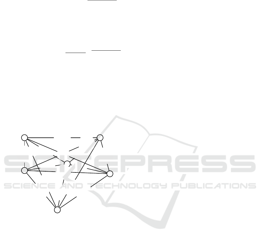
To assess the importance of incorporating cost
fluctuations in the problem, we present in Figure 1
a fictitious small example, including five potential
nodes to be visited. The ordered pair of over each
edge represents the expected cost and its standard de-
viation, respectively. The value under each node rep-
resents the revenue collected while visiting the node.
0
1
14
2
23
3
30
4
45
5
50
(16,1)
(10,7.0)
(24,1.5)
(19,1.37)
(35,1.8)
(24,1.55)
(23,1.51)
(22,1.48)
(47,2.16)
(23,1.51)
(16,2)
(24,7.7)
(7,2)
(36,1.89)
(30,8.36)
Figure 1: Network of example.
The solution of the deterministic PTP is the the tour
(0-2-5-4-3-0) with optimal objective function value
of 53 and a total variance of 186.4. When we con-
sider the EVaR risk measure with α = 0.01, we ob-
tain an optimal path (0-4-3-5-2-0) with a total vari-
ance of 119.5, which is much lower that the standard
deviation of the risk-neutral solution. In this case,
the decision-maker is willing to trade-off some profit
against less risky solutions.
The PTP is NP−hard even in the deterministic
case. The injection of uncertainty increases the com-
plexity of the problem, preventing the exact solution
within a reasonable time limit. In what follows, we
present two heuristic approaches for the risk averse
PTP. One is based on genetic algorithm and the other
is a tabu search heuristic.
4 HEURISTIC SOLUTION
APPROACHES
The Genetic Algorithm
A Genetic Algorithm (GA) is an evolutionary algo-
rithm that mimics the natural selection. A standard
GA starts with a population of encoded solutions
(chromosomes), which are initially, randomly gener-
ated. In our case, tours are encoded into two chromo-
somes as an ordered list of vertices serviced, as usual
in the TSP, and a list of not visited nodes. Each in-
dividual is then evaluated on the basis of the fitness
function φ which is simply the evaluation the objec-
tive function associated to the solution corresponding
to the encoding of the individual. We generate the
initial population randomly generating a number of
nodes to be visited (number of genes in the first chro-
mosome) and then by picking the value of each gene
from the standard uniform distribution in the range
[0,n]. The second chromosome is simply the list of
nodes not included in the first one. After the con-
struction of the initial population, the GA generates
a new set of individuals from the parent population,
applying the crossover operator on the first chromo-
some, which recombines parts of the parent informa-
tion. In our case the order crossover operator has been
applied. A tournament selection method for a parent
selection is used, which begins by forming two teams
of chromosomes. Each team consists of ten individu-
als randomly drawn from the current population. The
best individuals, selected from each of the two teams,
are then chosen for crossover operations. As such,
two offsprings are generated and entered into the new
population. The best solution at each iteration is im-
proved by applying the two-opt heuristic.
As a diversification mechanism, the GA may
employ a mutation operator which modifies a child
chromosome with a given probability. We imple-
mented two possible kinds of mutation: inserting a
new gene or removing an existing gene. In particular,
for each individual, the following procedure is
executed. For each node i ∈ V a random number is
generated between 0 and 1. If the random number is
below a given mutation probability π
mut
and the node
is present in the individual, it will be removed from
the tour, otherwise it will be added in the best position
in the tour. After the generation of the offspring,
some chromosomes in both the parent population and
the offspring are eliminated according to their relative
fitness function values. The remaining chromosomes
form a new population. The scheme of the GA is
reported in Algorithm 1.
ICORES 2019 - 8th International Conference on Operations Research and Enterprise Systems
462

Algorithm 1: The GA pseudo-code.
1 Input: π
mut
2 Initialization: best, currentbest := null;
P
curr
,P
best
=
/
0.
3 Create an initial population of |V | individuals
and store them in P
curr
. Evaluate the fitness
of the population.
4 repeat
5 P
it
= P
curr
6 P
cross
,P
mut
=
/
0
7 Apply the tournament selection method
to the population. Let the parents be the
best inidivduals in each tournament.
8 Apply the order crossover operator to the
parents, obtaining two new individuals
and apply the generational replacement.
for i ∈ P
it
do
9 for g = 1,...,|V | do
10 Generate a random value r in
(0,1).
11 if r <= π
mut
then
12 if g is in the chromosome list
of the individual i then
13 remove it
14 end
15 add g in the best position
16 end
17 end
18 end
19 it:=it+1
20 currentbest = argmin
i∈P
curr
φ
i
21 if φ
currbest
> φ
best
then
22 Apply two-opt. Update φ
best
23 end
24 until a given termination criterion is met;
25 Return φ
best
The TABU Search Algorithm. The first heuristic
is a tabu search heuristic (TS), inspired by the one
proposed in (Gendreau et al., 1998). This kind of
metaheuristic has been proved to be successful in
solving difficult routing problems (Guerriero et al.,
2013). Generally speaking, the TS systematically ex-
plores the solution space by moving at each iteration
from the current solution s to the best one amongst
its neighbours. To avoid cycling, solutions possess-
ing some attributes of recently explored solutions are
temporarily declared tabu (i.e. forbidden) and the
number of iterations an attribute remains tabu is de-
noted with θ.
The initial tour is built by a construction heuris-
tic which forms a tour of length
n
2
. First, the two
highest profit vertices are included in the tour T
and afterwards, in each successive iteration and un-
til the desired length is reached, two adjacent ver-
tices are randomly determined in the tour (let say i
and k) and a city j /∈ T having the minimal ratio
( ¯c
i j
+ ¯c
jk
− ¯cik)/p
j
, is added. The whole procedure
is repeated for five times, and best tour is retained.
Before starting with the tabu iterations, several parti-
tions of the node set V
0
are defined, each containing
one or more clusters of vertices. The first partition
contains n clusters, each containing one node. In any
successive partition two clusters (R,S) yielding the
minimum proximity measure ∆, are merged (in the
first iteration the clusters are singletons). The proxim-
ity measure between two clusters R and S is defined
as ∆(R,S) =
2
|R||S|
∑
i∈R, j∈S
¯c
i j
− Γ(R) − Γ(S), where
Γ(R) =
1
|R|(|R|−1)
∑
i, j∈R
¯c
i j
if the cluster has at least
two nodes and zero otherwise. Only partitions with a
number of nodes equal to n + 1 − 1,n + 1 − [n/2],n +
1 − [2n/3],n + 1 − [3n/4], . ..,n + 1 − [9n/10] are re-
tained. Then one partition is selected randomly and
each cluster belonging to the partition is evaluated.
The best cluster will be then selected to form the
neighbours of the current solution, obtained by two
possible moves. Either a move consists in inserting a
cluster of nodes in their best position in current solu-
tion or in removing a chain of nodes (a set of adjacent
nodes) from the current solution.
Each cluster is evaluated for insertion on the ba-
sis of the ratio of added profit over added distance.
In particular, the gravity centre is first computed for
all the clusters and a preliminary move evaluation is
made, for each cluster C according to the formula
∑
i
∈C
p
i
/∆
cost
, where ∆
cost
is the difference between
the expected cost of the tour, obtained by inserting
the gravity center in its best position, and the cost of
the tour without the gravity center.
Clusters of vertices candidate for removal
are defined as follows. Let consider a tour
{0,..., j
0
,i
1
,..., j
1
,i
2
,..., j
2
,i
3
..., j
λ−1
,i
0
,...,0}
where ( j
0
,i
1
),( j
1
,i
2
),...,( j
λ−1
,i
0
)) are the λ highest
cost edges of the tour. Then, the chains of adjacent
vertices are {(i
1
,..., j
1
),...,((i
λ−1
,..., j
λ−1
)}.
The value of a move associated with the removal
of a chain Ch is measured by the ratio of saved cost
over lost profit, and is computed as
∑
i
∈Ch
p
i
/∆
cost
,
where ∆
cost
is the difference between the expected
cost of the tour the cost of the tour obtained by taking
away the ordered subset of vertices belonging to the
chain and by connecting the endpoints of the route.
The results of the insertion and deletion are then com-
pared and the best move is applied. If the best move is
a deletion of a chain of nodes, then all the vertices of
the chain are declared tabu for θ iterations. A random
The Risk-averse Profitable Tour Problem
463

diversification mechanism is applied if the solution is
not improved after a given number of iterations, by
perturbing the current solution. An overall descrip-
tion of the tabu search algorithm is reported in Algo-
rithm 2.
Algorithm 2: The TABU pseudo-code.
1 Input: κ, θ
2 Initialization: best := −∞; it = 0
3 Generate an initial solution s and set s
min
:= s
4 Determine the partitions
5 Set λ = rand[2,max(4,n/2)],
θ = rand(5,25), κ = 5.
6 repeat
7 Evaluate all the clusters for insertions and
all the chains for deletions.
8 Choose the best move on the basis of the
evaluations and modify the solution s
accordingly if the best move is a
deletion then
9 identify the tabu set T(s) forbidding
for the next θ iterations the nodes of
the selected chain
10 end
11 if it mod κ = 0 then
12 apply two-opt
13 end
14 Evaluate the objective function value of s,
OF(s). if s improves the previous best
known solution then
15 apply 3-opt and set best := OF(s)
16 end
17 if no improvement after 100 iterations
then
18 shuffle the route
19 end
20 it:=it+1
21 until a given termination criterion is met;
22 Return best
5 COMPUTATIONAL RESULTS
In this Section we discuss the numerical results
obtained by applying the two algorithms. All the
heuristics were implemented in Python 3 and run
on a laptop with an Intel(R) 4 Core (TM) i7-4600U
CPU with 8 Gb RAM and 64-bit operating system.
Then, we test the performance of the TABU and
the GA presented in Section 4 and identify the best
solution method to be used in the more extensive
numerical tests presented in the last part of the Sec-
tion. We performed the experiments on 57 instances
Table 1: GA versus TABU.
Instance Nodes # Visited GA # Visited TABU %Impr
a280.tsp 280 272 151 66,77
ali535.tsp 535 534 267 64,33
berlin52.tsp 52 46 45 -5,24
bier127.tsp 127 122 112 5,40
ch130.tsp 130 125 123 4,05
ch150.tsp 150 143 129 16,62
d198.tsp 198 194 153 29,21
d493.tsp 493 492 246 77,52
d657.tsp 657 656 328 72,79
dsj1000.tsp 1000 998 500 52,72
eil101.tsp 101 92 92 -3,66
eil51.tsp 51 37 42 -19,43
eil76.tsp 76 65 65 -1,21
fl417.tsp 417 414 208 87,82
gil262.tsp 262 261 147 61,40
gr137.tsp 137 135 124 5,02
gr202.tsp 202 199 163 18,46
gr229.tsp 229 228 177 22,65
gr431.tsp 431 430 215 86,21
gr666.tsp 666 665 333 86,00
gr96.tsp 96 92 93 -1,43
kroA100.tsp 100 94 98 -0,93
kroA150.tsp 150 145 139 4,06
kroA200.tsp 200 196 130 40,77
kroB100.tsp 100 96 97 -0,62
kroB150.tsp 150 146 132 9,76
kroB200.tsp 200 197 133 43,09
kroC100.tsp 100 94 96 0,40
kroD100.tsp 100 95 97 -1,38
kroE100.tsp 100 96 95 -0,24
lin105.tsp 105 102 104 -0,58
lin318.tsp 318 316 159 74,35
linhp318.tsp 318 315 159 69,90
p654.tsp 654 653 327 79,83
pcb442.tsp 442 441 221 71,55
pr107.tsp 107 103 103 -0,13
pr124.tsp 124 123 122 -0,54
pr136.tsp 136 132 128 2,49
pr144.tsp 144 142 132 4,74
pr152.tsp 152 150 140 6,41
pr226.tsp 226 221 133 46,26
pr264.tsp 264 256 150 62,72
pr299.tsp 299 295 159 75,81
pr439.tsp 439 438 219 73,08
pr76.tsp 76 72 72 -4,86
rat195.tsp 195 191 141 31,36
rat575.tsp 575 574 287 75,99
rat783.tsp 783 782 391 78,00
rat99.tsp 99 93 95 0,40
rd100.tsp 100 94 89 0,30
rd400.tsp 400 397 200 48,80
st70.tsp 70 60 63 -0,81
ts225.tsp 225 215 136 50,19
tsp225.tsp 225 217 134 47,72
u159.tsp 159 155 144 2,94
u574.tsp 574 573 287 79,75
u724.tsp 724 723 362 74,84
taken from the TSPLIB htt ps : //www.iwr.uni − hei
delberg.de/groups/comopt/so f tware/T SPLIB95/
with a number of nodes ranging from 51 to 1000
nodes. To create the test instances, we considered
the random cost ˜c
i j
= ξ ∗ ¯c
i j
, where the nominal
cost over the edge (i j) has been set proportional to
the Euclidean distance between node i and j and ξ
is a normal random variable with given mean and
variance. For both the algorithms a time limit of 60
ICORES 2019 - 8th International Conference on Operations Research and Enterprise Systems
464
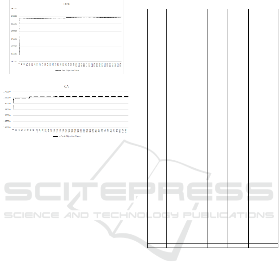
Figure 2: Iterations of the TABU.
Figure 3: Iterations of the GA.
seconds has been imposed. In the Table 1, we report
the name of the instances, the number of nodes, the
number of nodes visited in the solutions provided by
the algorithms and the percentage Improvement of
GA versus TABU (column heading %Impr).
As evident, the GA is able to find better solu-
tions than the TABU and the average improvement
is around 33%. This is due to the nature of the GA
which works with a a pool of complete solutions and
not to the specific choice of the operators, which have
not been tailored for the problem at hand. In 44 out
of 57 instances, the GA finds tours visiting a higher
number of nodes. When the TABU is able to outper-
form the GA (and a negative value of the percentage
improvement is reported in the dedicated column) the
number of visited nodes is equal or very close for both
the methods. Analyzing more in detail the behaviour
of the algorithms for a given instance (gr96.tsp) we
notice, from Figures 2 and 3 that the GA performs a
lower number of iterations (less than one third) than
the TABU. Both algorithms are able to obtain a good
solution after half of the total number of iterations,
i.e. the TABU which reaches a good solution after
around 900 iterations out of 1834. In Table 2 is re-
ported the deviation of the solution values of the five
random runs for the GA. The last column %∆ repre-
sents the percentage deviation between the maximum
and minimum value of the objective function. This
variability of the solutions arises from the choice of
the random seeds, and from the randomness involved
in the algorithm. This information is important to as-
sess how robust the heuristic is in terms of the solution
consistency.
Table 2: Performance of the GA with differents seeds.
Instance Seed 4 Seed 5 Seed 6 Seed 7 Seed 8 %∆
a280.tsp 5516133 5512424 5515533 5512693 5508237 0.14
ali535.tsp 22147713 22088638 22113013 22125713 22178113 0.41
berlin52.tsp 544107 544107 557231 559231 553331 2.78
bier127.tsp 65511768 65334239 64990332 65348039 65466639 0.80
ch130.tsp 3186711 3193691 3193691 3193591 3193691 0.22
ch150.tsp 4150750 4156098 4156998 4147736 4162735 0.36
d198.tsp 38627538 38640059 38631623 38644618 38638512 0.04
d493.tsp 252483148 252511548 252579548 252325790 252414367 0.10
d657.tsp 500782552 501218840 500881452 500886852 500976952 0.09
dsj1000.tsp 2.85261E+11 2.85261E+11 2.84993E+11 2.85108E+11 2.85245E+11 0.09
eil101.tsp 167737 172142 172642 172173 172928 3.09
eil51.tsp 12526 14362 14429 14516 13643 15.89
eil76.tsp 63308 63308 61345 62509 63302 3.20
fl417.tsp 104316634 104082283 104241883 104179591 104119883 0.23
gil262.tsp 4278023 4353026 4366527 4342957 4353671 2.07
gr137.tsp 682127 682227 678682 682427 682527 0.57
gr202.tsp 1089744 1090779 1091272 1090723 1090525 0.14
gr229.tsp 4415630 4415232 4416198 4416756 4413990 0.06
gr431.tsp 17558075 17555108 17557575 17556375 17556475 0.02
gr666.tsp 39501237 39493137 39515237 39488537 39497537 0.07
gr96.tsp 166044 166044 165485 166088 166013 0.36
kroA100.tsp 7941865 7904464 7793754 7874520 7931956 1.90
kroA150.tsp 21921673 22042335 22012635 21769024 21940948 1.26
kroA200.tsp 44769001 44779766 44771573 44608987 44451500 0.74
kroB100.tsp 6914730 6873487 6750118 6923030 6931382 2.69
kroB150.tsp 20240863 20307834 20116971 20019636 20297334 1.44
kroB200.tsp 35893778 35669586 35873276 35893471 35721935 0.63
kroC100.tsp 9171848 9099833 9089433 9015458 9074246 1.73
kroD100.tsp 7529474 7328771 7438351 7570674 7441974 3.30
kroE100.tsp 7264044 7211989 7161467 7290844 7265835 1.81
lin105.tsp 7106445 7055818 7106445 7075044 7101645 0.72
lin318.tsp 116486420 116785931 116720784 116892758 116846162 0.35
linhp318.tsp 113003012 113224770 113168804 113100132 113411282 0.36
p654.tsp 661050147 661458847 661284647 661080447 660779924 0.10
pcb442.tsp 221321761 221486561 221859161 221362445 221726061 0.24
pr107.tsp 25328948 25328948 25333251 25319748 25346848 0.11
pr124.tsp 46923397 46759814 46880997 47048723 46536753 1.10
pr136.tsp 53805109 53859976 53796729 53669821 53844885 0.35
pr144.tsp 56556141 56556141 56387341 56556141 56556141 0.30
pr152.tsp 84640652 84812508 84556837 84737764 84812508 0.30
pr226.tsp 204150277 204281100 204258422 203941226 204211768 0.17
pr264.tsp 146436552 146214768 146112774 145891647 146657398 0.52
pr299.tsp 151796427 152291132 152388830 152064812 151949428 0.39
pr439.tsp 595473482 597012382 596142083 596290682 596011082 0.26
pr76.tsp 19250820 18907065 19245511 19250820 19250820 1.82
rat195.tsp 2724185 2729911 2727943 2727183 2729562 0.21
rat575.tsp 43644365 43598665 43598765 43581265 43626765 0.14
rat783.tsp 92716430 92720043 92704330 92669430 92724730 0.06
rat99.tsp 386922 388434 388434 387754 388434 0.39
rd100.tsp 2236314 2236089 2224455 2163871 2225658 3.35
rd400.tsp 48288473 48256500 48547371 48542071 48941571 1.42
st70.tsp 90498 90434 90453 90434 90173 0.36
ts225.tsp 198420303 198026821 198684376 198553972 198729501 0.35
tsp225.tsp 6075338 6066911 6066092 6027446 6054097 0.79
u159.tsp 35047328 35084536 35084536 35050936 35050936 0.11
u574.tsp 272905885 272996985 272926018 272982185 272982085 0.03
u724.tsp 395250080 395429945 395306980 395237331 395381080 0.05
1.06
From the observation of the results we notice that
the relative deviation of the GA is quite small and on
average around 1%. This implies that GA best fitness
value fluctuates only slightly around the best solution
identified by the same algorithm.
6 CONCLUSIONS
In this paper, we have presented an interesting variant
of the profitable tour problem with stochastic costs
under a risk.-averse perspective. We have developed
two metaheuristics based on a GA and a TABU search
method, respectively to solve the problem. Future
work can be directed along the following directions.
First, we can assume that different edges may have
different correlated costs. This situation can be rele-
vant, especially in disaster management applications.
The Risk-averse Profitable Tour Problem
465

Second, advanced heuristics in the spirit of adaptive
large neighborhood search heuristics may be devised.
REFERENCES
Ahmadi-Javid, A. (2012a). Addendum to: Entropic value-
at-risk: A new coherent risk measure. J. Optimization
Theory and Applications, 155(3):1124–1128.
Ahmadi-Javid, A. (2012b). Entropic value-at-risk: A new
coherent risk measure. J. Optimization Theory and
Applications, 155(3):1105–1123.
Archetti, C., Speranza, M., and Vigo, D. (2013). Vehi-
cle routing problems with profits. WPDEM 2013/3-
Working Papers Department of Economics and Man-
agement University of Brescia Italy.
Balas, E. (1995). The prize collecting traveling salesman
problem. ii: Polyhedral results. Networks, 25:199–
216.
Beraldi, P., Bruni, M. E., Lagan
`
a, D., and Musmanno, R.
(2015a). The mixed capacitated general routing prob-
lem under uncertainty. European Journal of Opera-
tional Research, 240(2):382–392.
Beraldi, P., Bruni, M. E., Lagann
`
a, D., and Musmanno, R.
(2019). The risk-averse traveling repairman problem
with profits. Soft Computing, in press.
Beraldi, P., Bruni, M. E., Manerba, D., and Mansini, R.
(2015b). A stochastic programming approach for the
traveling purchaser problem. IMA Journal of Manage-
ment Mathematics, 28(1):41–63.
Beraldi, P., Bruni, M. E., and Violi, A. (2012). Capital ra-
tioning problems under uncertainty and risk. Compu-
tational Optimization and Applications, 51(3):1375–
1396.
Bruni, M. E., Beraldi, P., and Khodaparasti, S. (2018a). A
fast heuristic for routing in post-disaster humanitar-
ian relief logistics. Transportation Research Procedia,
30:304–313.
Bruni, M. E., Beraldi, P., and Khodaparasti, S. (2018b). A
heuristic approach for the k-traveling repairman prob-
lem with profits under uncertainty. Electronic Notes
in Discrete Mathematics, 69:221–228.
Bruni, M. E., Guerriero, F., and Beraldi, P. (2014). De-
signing robust routes for demand-responsive transport
systems. Transportation Research Part E: Logistics
and Transportation Review, 70(1):1–16.
Campbell, A., Gendreau, M., and Thomas, B. (2011). The
orienteering problem with stochastic travel and ser-
vice times. Annals of Operations Research, 186:61–
81.
Chao, I., Golden, B., and Wasil, E. (1996). A fast and effec-
tive heuristic for the orienteering problem. European
Journal of Operational Research, 88:475–489.
Cominetti, R. and Torrico, A. (2016). Additive consistency
of risk measures and its application to risk-averse rout-
ing in networks. Mathematics of Operations Research,
41(4):1510–1521.
Dell’Amico, M., Maffioli, F., and Sciomachen, A. (1998). A
lagrangian heuristic for the prize collecting travelling
salesman problem. Annals of Operations Research,
81:289–306.
Dell’Amico, M., Maffioli, F., and Varbrand, P. (1995). On
prize-collecting tours and the asymmetric travelling
salesman problem. International Transactions in Op-
erational Resesarch, 2(3):297—-308.
Evers, L., Glorie, K., Van Der Ster, S., Barros, A. I., and
Monsuur, H. (2014). A two-stage approach to the ori-
enteering problem with stochastic weights. Comput-
ers and Operational Research, 43:248–260.
Feillet, D., Dejax, P., and Gendreau, M. (2009). Traveling
salesman problems with profits. Transportation Sci-
ence, 39(2):188–205.
Fischetti, M., Gonz
´
alez, J. S., and Toth, P. (1998). Solv-
ing the orienteering problem through branch-and cut.
INFORMS Journal on Computing, 10:133–148.
Fischetti, M. and Toth, P. (1988). An additive approach for
the optimal solution of the prize-collecting traveling
salesman problem. In Vehicle Routing: Methods and
Studies, page 319–343. B.L. Golden and A.A. Assad,
editors.
Gendreau, M., Laporte, G., and Semet, F. (1998). A tabu
search heuristic for the undirected selective travelling
salesman problem. European Journal of Operational
Research, 106:539–545.
Guerriero, F., BRUNI, M. E., and GRECO, F. (2013). A
hybrid greedy randomized adaptive search heuristic to
solve the dial-a-ride problem. Asia-Pacific Journal of
Operational Research, 30(01):1250046.
JF. Berube, M. G. and Potvin, J. (2009). A branch-and-cut
algorithm for the undirected prize collecting traveling
salesman problem. Networks, 54:56–67.
Klau, G. W., Ljubic, I., Moser, A., Mutzel, P., Neuner,
P., Pferschy, U., Raidl, G. R., and Weiskircher, R.
(2004). Combining a memetic algorithm with inte-
ger programming to solve the prize-collecting steiner
tree problem. In GECCO (1), volume 3102 of Lec-
ture Notes in Computer Science, pages 1304–1315.
Springer.
Leitner, M., Ljubic, I., Gonz
´
alez, J. J. S., and Sinnl, M.
(2017). An algorithmic framework for the exact solu-
tion of tree-star problems. European Journal of Oper-
ational Research, 261(1):54–66.
˙
Ilhan, T., Iravani, S. M. R., and Daskin, M. S. (2008).
The orienteering problem with stochastic profits. IIE
Transactions, 40(4):406–421.
Millar, H. H. and Kiragu, M. (1997). A time-based for-
mulation and upper bounding scheme for the selective
traveling salesperson problem. Journal of the Opera-
tional Research Society, 48:511–518.
Ogryczak, W. and Ruszczy
´
nski, A. Dual stochastic dom-
inance and quantile risk measures. International
Transactions in Operational Research, 9(5):661–680.
Ramesh, R., Yoon, Y.-S., and Karwan, M. (1992). An
optimal algorithm for the orienteering tour problem.
ORSA Journal on Computing, 4:155–165.
Rockafellar, R. T. and Uryasev, S. (2002). Conditional
value-at-risk for general loss distributions. Journal of
Banking and Finance, pages 1443–1471.
Tang, H. and Miller-Hooks, E. (2005). Algorithms for
a stochastic selective travelling salesperson prob-
lem. Journal of the Operational Research Society,
56(4):439–452.
ICORES 2019 - 8th International Conference on Operations Research and Enterprise Systems
466
