Grid-based Exploration of OCT Thickness Data of Intraretinal Layers

Martin R

ohlig

, J

org St

uwe

, Christoph Schmidt

, Ruby Kala Prakasam

, Oliver Stachs

and Heidrun Schumann

Institute of Computer Science, University of Rostock, Albert-Einstein-Str. 22, Rostock, Germany

Department of Ophthalmology, University of Rostock, Doberaner Str. 140, Rostock, Germany

Keywords:

Visual Analysis of OCT Data, Optical Coherence Tomography, Modiﬁed ETDRS Grids, Intraretinal Layers.

Abstract:

Optical coherence tomography (OCT) enables high-resolution 3D imaging of the human retina to understand

a variety of retinal and systemic disorders. Commonly, the thickness of segmented intraretinal layers is used to

assess the condition of the retina. However, the thickness data are complex and thus, need to be considerably

reduced prior to further processing and analysis. This leads to a loss of information and may hinder the

discovery of subtle and localized retinal changes, which are important for an early detection of certain diseases.

On this account, we propose an enhanced grid-based reduction of OCT thickness data. We adapt established

grid types for retinal thickness data and suggest alternative grids that capture more information. We integrate

our data reduction approach into a visual analysis tool that supports an automated computation and interactive

exploration of different grids. We demonstrate the application of our tool and show how it can be used to

support experts in choosing and comparing appropriate grid representations for given OCT thickness data.

1 INTRODUCTION

Optical coherence tomography (OCT) is a widely-

used noninvasive technique to capture high-resolution

3D images of retinal substructures. Ophthalmolo-

gists analyze the resulting data to understand a va-

riety of retinal and systemic disorders, e.g., diabe-

tic retinopathy, age-related macular degeneration, and

glaucoma. Particularly, the thickness of segmented

intraretinal layers is used to assess the condition of

the retina. However, derived thickness data are com-

plex, as one thickness value is typically computed for

every single point of each intraretinal layer. On the

one hand, this enables a spatially precise judgment of

the layers. On the other hand, the large amounts of

thickness values are difﬁcult to deal with, and a ge-

neral summary of thickness changes in larger retinal

areas is missing. Hence, ophthalmologists typically

rely on considerable data reduction prior to further

processing and analysis of the data.

Established data reduction approaches for OCT

thickness data are commonly based on retinal grids.

These grids are used to spatially divide the retina into

few large regions and to derive aggregated thickness

measures for each region. This helps to get a quick

overview of the layers’ thickness in anatomically pre-

deﬁned areas. Moreover, it drastically reduces the

amount of information to be analyzed, particularly if

the layer thickness in larger studies with dozens or

hundreds of OCT datasets has to be evaluated. Yet,

due to the spatial aggregation, information loss may

occur. This is because small and localized variations

in thickness are not always reasonably represented via

aggregated values of large regions. Capturing such in-

formation is, however, mandatory for detecting early

signs of certain diseases or investigating progressions.

We aim at supporting ophthalmologists in their

grid-based visual analysis of intraretinal layer

thickness. We propose an enhanced data reduction

scheme together with a visual analysis tool for the ex-

ploration of alternative grids. Our approach helps to

strike a balance between obtaining a compact grid re-

presentation of thickness data and being able to cap-

ture more relevant information of intraretinal layers.

Our contributions are:

New Grid Design: We propose an enhanced grid-

based reduction scheme for OCT thickness data.

New grid layouts are derived based on radial and

sector-wise subdivision of well-established grids.

Data-driven Adaptation: We introduce a procedure

to compute the suitability of different grid layouts

for given thickness data. The grids are rated and

best options are suggested to the user.

Röhlig, M., Stüwe, J., Schmidt, C., Prakasam, R., Stachs, O. and Schumann, H.

Grid-based Exploration of OCT Thickness Data of Intraretinal Layers.

DOI: 10.5220/0007580001290140

In Proceedings of the 14th International Joint Conference on Computer Vision, Imaging and Computer Graphics Theory and Applications (VISIGRAPP 2019), pages 129-140

ISBN: 978-989-758-354-4

129

Grid-based Exploration: We develop a new vi-

sual analysis tool for grid-based exploration of

thickness data. Grids are interactively adjusted,

compared to other grids of different datasets, and

grid-related details are investigated on demand.

2 BACKGROUND

Our work is motivated and driven by advances in the

detection of retinal diseases. Particularly, the dyna-

mic development of OCT technology with respect to

image quality, e.g., the improvement of the axial and

lateral resolution, offers a unique possibility of dif-

ferentiating and precisely measuring substructures of

the retina. Modern OCT devices are able to capture

even subtle retinal changes and allow to accurately

monitor the progression of a disease. Based on the

data, ophthalmologists aim at performing both:

• Patient-speciﬁc assessments of the retinal condi-

tion of individuals

• Group-speciﬁc evaluations of experimental and

prospective studies in ophthalmic research

In this context, they often need to compare multi-

ple intraindividual datasets, e.g., follow-up examina-

tions of a single patient, and interindividual datasets,

e.g., examinations of patients in relation to normative

data of controls. Yet, the data analysis can be complex

and the available analysis methods differ between ex-

isting software tools. In this regard, our work is rela-

ted to the visual analysis of retinal OCT data in gene-

ral, and to the representation of retinal layer thickness

via grids in particular.

2.1 Visual Analysis of OCT Data

Current analysis procedures are based on a combina-

tion of commercial OCT software, non-commercial

OCT software, and general-purpose analysis soft-

ware. Segmentation of intraretinal layers and measu-

rement of layer thickness are supported by both com-

mercial software and non-commercial software (Gar-

vin et al., 2009; Mayer et al., 2010; Mazzaferri et al.,

2017). Commercial OCT software is commonly dis-

tributed by OCT device manufactures. Currently, se-

veral major platforms are available, including soft-

ware from Nidek, Optovue, Zeiss, Topcon, Heidel-

berg Engineering and others. The provided software

platforms are predominantly used in clinical practice

as well as for ophthalmic research. Besides commer-

cial software, few approaches for visually analyzing

retinal OCT data exist. Examples are the research-

oriented Iowa Reference Algorithms (Garvin et al.,

2009), the open-source software ImageJ (Schindelin

et al., 2015) and its application to OCT data (Garrido

et al., 2014), a 3D visualization of OCT data based on

ray-tracing (Glittenberg et al., 2009), and a recent vi-

sual analysis framework based on multiple coordina-

ted views (R

ohlig et al., 2018). These software tools

are typically applied in ophthalmic research. In gene-

ral, all available analysis software packages support at

least one of three fundamental presentation methods

for OCT data: cross-sectional views, 3D views, and

top-down views.

Cross-sectional views show individual 2D image

slices of volumetric OCT data together with overlaid

proﬁles of segmented intraretinal layers. This allows

to view details but ﬂipping through the images is time-

consuming, as OCT datasets can consist of hundreds

of slice images. 3D views show an entire OCT dataset

as a 3D volume rendered tomogram. This provides

an overview of the data but combined 3D visualizati-

ons of the tomogram and the layers are only provided

by few tools, e.g., (R

ohlig et al., 2018). Top-down

views show a fundus image of the interior surface of

the eye around the OCT acquisition area together with

superimposed retinal layers. This facilitates a layer-

centric analysis of the data and helps to link the lay-

ers to retinal areas in the fundus image. In general,

cross-sectional views and 3D views are mainly used

for the visual analysis of individual datasets, whereas

top-down views are also applied to anatomically lo-

calize and compare areas under investigation in mul-

tiple OCT datasets. In this regard, top-down views are

most relevant to our work.

Instead of showing the raw OCT data, top-down

views typically represent intraretinal layers via their

derived layer thickness. The layer thickness is dis-

played either via thickness maps or via spatially

aggregated thickness grids. This helps to reveal

even subtle retinal changes, which may be difﬁcult

to identify by visualizing the raw OCT data alone.

While there recently have been advances in the ap-

plication of thickness maps for the analysis of OCT

data (R

ohlig et al., 2018), thickness grids are still pre-

dominantly used in most opthalmic applications. On

the other hand, the design of thickness grids has been

hardly investigated in previous work, despite the con-

tinuous development of OCT technology and asso-

ciated analysis methods. On this account, we parti-

cularly focus on the grid-based exploration of retinal

thickness data.

IVAPP 2019 - 10th International Conference on Information Visualization Theory and Applications

130

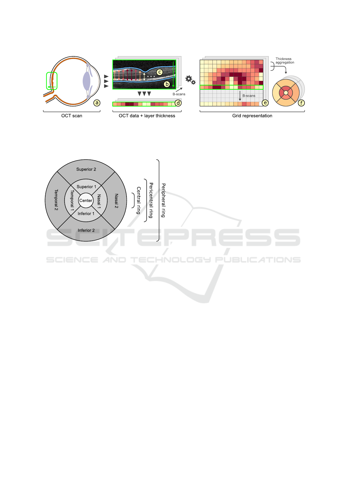
Figure 1: Grid representation of retinal layer thickness. An OCT scan captures the area around the macula and the optic

disk (a). The resulting volumetric data consists of multiple 2D image slices (B-scans) (b). Several intraretinal layers are ex-

tracted from each B-scan (c) and thickness values are computed for every pixel along the horizontal image axes by measuring

the vertical distance between the upper and lower layer boundaries (d). The thickness values are combined across all B-scans

per retinal layer (e) and spatially aggregated into corresponding grid representations (f).

Figure 2: The layout of the ETDRS grid. The grid divides

the retina into nine regions deﬁned by three rings, i.e., cen-

tral, pericentral, and peripheral, and four sectors, i.e., nasal,

temporal, superior, and inferior.

2.2 Representation of Retinal Layer

Thickness via Grids

The most common grid type to represent retinal

thickness data was established by the Early Treatment

Diabetic Retinopathy Study (ETDRS) (Chew et al.,

1996). The cells of ETDRS grids divide the retina into

nine large regions, i.e., a central foveal ring with 1mm

diameter, an inner macula ring (pericentral) with 3mm

diameter, and an outer macula ring (peripheral) with

6mm diameter. The inner and outer rings are further

divided into four quadrants, namely nasal, temporal,

superior, and inferior. For each grid cell and intrare-

tinal layer, typically one aggregated thickness measu-

rement is stored. Figure 1 illustrates how such grid re-

presentations are obtained and Figure 2 shows the la-

yout of the ETDRS grid. The grid design enables the

localization and assessment of anatomically impor-

tant areas of the macula near the center of the retina.

Thus, ETDRS grids have been widely applied for va-

rious purposes in ophthalmic research, including in-

vestigations of early structural changes of the retina

for a variety of diseases, e.g., diabetes mellitus (G

otze

et al., 2018) and glaucoma (Chen et al., 2017). Alt-

hough other grid types exist, they have been mos-

tly designed for special applications, e.g., rectangular

grids for asymmetry analysis of retinal thickness for

glaucoma diagnosis (Asrani et al., 2011).

A major advantage of ETDRS grids is their com-

pact representation of the complex thickness data with

only few aggregated values for each intraretinal layer,

i.e., typically one arithmetic mean thickness value per

grid cell. This allows a quick overview and judgment

of thickness changes in predeﬁned retinal areas. Mo-

reover, the applied data reduction eases the evalua-

tion and comparison of multiple datasets. Particularly

in case of larger studies, it is easier to handle fewer

data values for statistical analysis and interpretation

of the data. That is because ophthalmologists conven-

tionally export ETDRS thickness values from OCT

software to external spreadsheet software or statistics

software to compile study groups and to perform ba-

tched or non-batched statistical analyses. On top of

that, the ﬁxed grid cells enable the comparison of re-

sults from different studies that used ETDRS grids.

On the downside, the main problem with ETDRS

grids is that they do not necessarily faithfully repre-

sent underlying thickness data (Fig. 3). Due to the

considerable spatial data reduction, localized variati-

ons in thickness of an intraretinal layer are not accu-

rately captured via a single aggregated thickness va-

lue per grid cell. This is the case for both small vari-

ations in thickness within a grid cell and variations

divided by the boundary of two or more grid cells

(Fig. 3c). Moreover, when evaluating deviations bet-

ween thickness data of multiple OCT datasets, aggre-

gation artifacts may bear an additional risk of infor-

mation loss. The reason for this is that localized po-

sitive and negative deviations within a grid cell may

be nulliﬁed during data reduction (Fig. 3g). This can

Grid-based Exploration of OCT Thickness Data of Intraretinal Layers

131

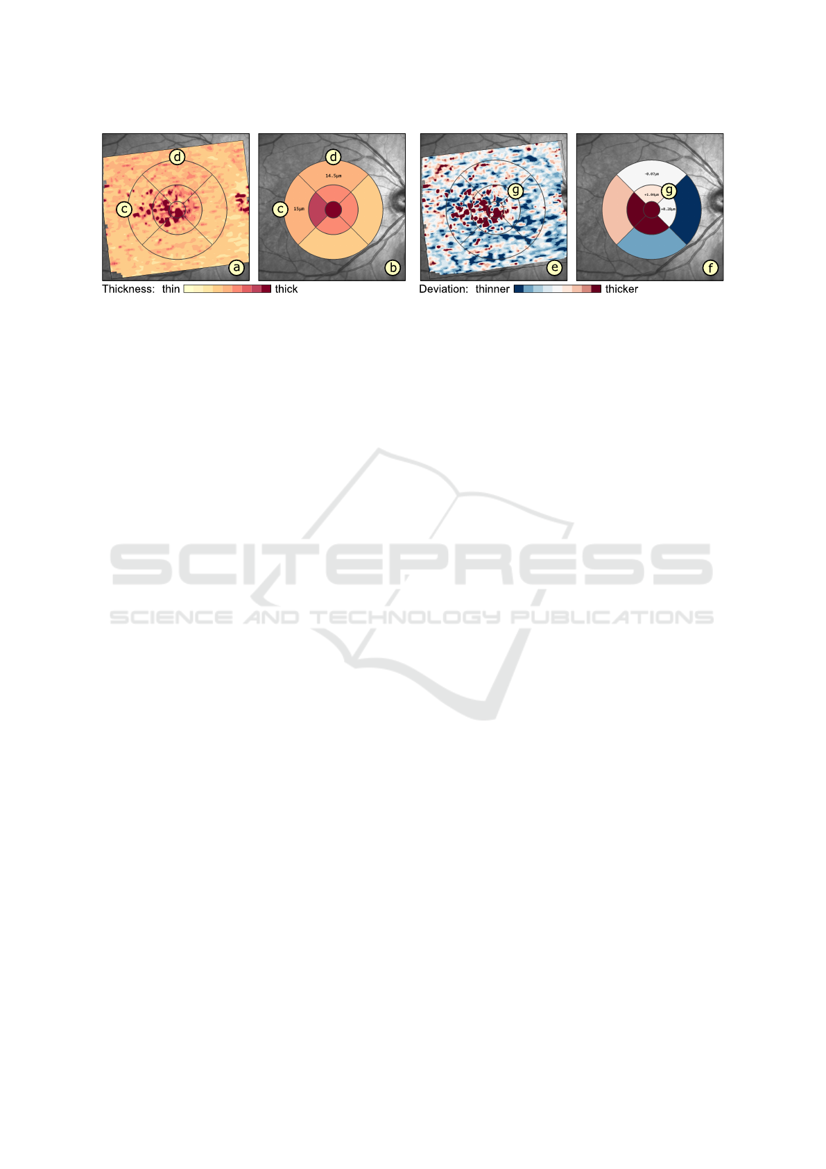
Figure 3: Data representation with ETDRS grids. The thickness of an intraretinal layer is shown via a thickness map (a) and

an ETDRS grid (b). Small and localized regions of high thickness (dark red) in the map are not accurately represented in all

cells of the grid, e.g., cell (c) with regions of high thickness has almost the same aggregated value as cell (d) without such

regions. In addition, localized regions of positive and negative deviations in thickness (dark red and dark blue) in the map (e)

are nulliﬁed in certain cells of the grid (f), e.g., averaging artifacts of grids cells (g).

lead to false normal ﬁndings. Detecting such infor-

mation is, however, vital for the identiﬁcation of early

retinal changes of certain diseases.

3 GRID DESIGN

Given both the discussed beneﬁts and drawbacks of

ETDRS grids, we aim at designing alternative grids

that combine the advantages of ETDRS grids with the

possibility to capture more relevant information. To

this end, we identiﬁed design requirements, devised a

new subdivision scheme that allows to compare diffe-

rent grid layouts, and developed a method to rate the

representation quality of grids for given data.

3.1 Requirements

The grid-related design requirements reﬂect the ex-

perts’ needs with regard to processing and analyzing

OCT thickness data. We derived the following list by

talking with the experts about current limitations and

about the way they utilize existing grids to analyze

thickness data of intraretinal layers.

Layout based on ETDRS Grid (GR

): The basic

layout of alternative grids should correspond to

the ETDRS grid. This is to maintain the ability

to localize anatomically important areas of the

macula near the center of the retina.

Compact Data Representation (GR

): In general,

the number of grid cells should be small and the

content of a grid cell should be mainly represen-

ted by only a single descriptive value. Nevert-

heless, an appropriate representation of thickness

data should be facilitated.

Compariability of Grid Layouts (GR

Alternative grid layouts should be compara-

ble to both the basic ETDRS grid and other

alternative grids. This is to ensure that analysis

results from multiple datasets with different grids

are relatable.

3.2 Subdivision of Grids

Based on the experts’ demands, we design alterna-

tive grids that meet requirements GR

and GR

. Our

approach is based on subdivisions of existing grid la-

youts. Taking the ETDRS grid as a basis, we employ

a radial or a sector-wise partition strategy of ETDRS

grid cells. This allows us to obtain alternative grids

that represent the underlying thickness data at diffe-

rent levels of granularity. Figure 4a exempliﬁes both

partition strategies.

Radial partitions add rings to a grid. The resulting

grid cells enable a more ﬁne-grained analysis of areas

with respect to the distance from the foveal center.

For example, intraretinal layer thickness of macula

rings can be investigated in-depth via secondary peri-

central or peripheral cells. Sector-wise partitions add

separating lines at certain angles to a grid. The ge-

nerated grid cells facilitate a more direction-centric

analysis of areas with respect to the foveal center.

For example, by adding further directional cells, the

thickness of areas facing nasally may be evaluated in

greater detail in relation to areas facing temporally.

Radial and sector-wise partitions can also be combi-

ned to obtain ﬁne grids that support analyses with fo-

cus on both properties.

To restrict the number of all possible combinati-

ons of subdivisions, we suggest to start by equally di-

viding grid cells and to increase the number of radii

or sectors in power of two steps. By dividing grid

cells in half for each radial or sector-wise subdivision

IVAPP 2019 - 10th International Conference on Information Visualization Theory and Applications

132

Figure 4: Subdivision and mapping of grids. The ETDRS

grid layout is subdivided via radial (dashed line) or sector-

wise (dotted line) partitions to derive alternative grids (a).

To ensure the comparability of grids, a coarse grid is map-

ped to a ﬁne grid or vice versa by subdividing or merging

corresponding grid cells (b).

pass, the amount of information stored in a subdivi-

ded grid is increased in constant steps. The resulting

set of grids can then be reﬁned interactively. Just like

conventional ETDRS grids, we represent the content

of each grid cell via one aggregated thickness mea-

surement. Optionally, additional summary statistics,

e.g., mean, percentiles, and standard deviation, may

be stored per cell to provide further information on

the distribution of the underlying thickness data.

Utilizing the well-known ETDRS grid as a basis

for radial or sector-wise subdivisions helps experts

to familiarize themselves with the layout of derived

grids. The simple and ﬁxed subdivision scheme eases

the localization of areas under investigation and the

interpretation of the data. This in turn increases the

acceptance of alternative grids. Next, we discuss how

to further support experts in choosing an appropriate

grid from a set of alternatives for their given data.

3.3 Rating of Grids

In general, no single grid layout exists that ﬁts all pos-

sible spatial distributions of thickness data. Instead of

trying to create such an all-solving solution, we pro-

vide a set of alternative grids to choose from. Yet,

given all available grid layouts, experts now face the

problem that they have to decide which grid actually

matches their given data. To support experts in this

decision, we developed a rating procedure based on

a quantitative measure of the representation quality

for each grid under consideration. With our rating of

grids we are able to address the second aspect of de-

sign requirement GR

We determine the overall representation quality of

a grid by measuring the homogeneity of thickness va-

lues of all data points within each grid cell. This is

based on the assumption that a cell with high homo-

geneity covers thickness values that are more or less

equal, whereas a cell with low homogeneity encloses

strongly varying thickness values. Thus, an aggrega-

ted thickness value of a grid cell with high homoge-

neity matches the thickness values within that cell. In

contrast, a cell with low homogeneity indicates infor-

mation loss, e.g., due to averaging of localized vari-

ations. Consequently, a grid composed of cells with

high homogeneity corresponds to a good representa-

tion of the underlying thickness data and vice versa.

One possible measure to quantify the amount of

variation or homogeneity of a set of thickness values

inside a grid cell is the standard deviation. Based on

this simple measure, we obtain the overall rating of a

grid via the weighted arithmetic mean of the compu-

ted standard deviations of all grid cells.

x =

∑

i=1

∑

i=1

In this equation, x represents the ﬁnal rating of the

grid, n denotes the number of grid cells, x

is the stan-

dard deviation of a cell, and w

is the weight for that

cell given by the normalized amount of enclosed data

points (equal to the size of the cell). Based on the ﬁnal

ratings, we compute a ranking for a set of alternative

grids and suggest a best ﬁt for thickness data of one

retinal layer while considering secondary expert con-

straints. Such constraints are a speciﬁed maximum

number of allowed grid cells or a preference for either

radial or sector-wise subdivisions. This promotes a

more patient-speciﬁc analysis in contrast to generali-

zing all given thickness data to just the ETDRS grid

representation. Likewise, the rating and ranking can

be adapted to support a group-speciﬁc assessment of

grids. The procedures allow to ﬁnd one best ﬁtting

grid for multiple layers of one dataset or even for one

or several layers of multiple datasets, e.g, to obtain

one grid to represent the data of all patients in a study.

The resulting rankings are then used to steer the grid-

based visual exploration of thickness data.

3.4 Comparability of Grids

Ophthalmologists are often interested in relating

grid-based analysis results from multiple datasets

(cf. GR

). In a patient-speciﬁc analysis scenario, each

of these individual datasets may be best represented

by another grid with a different layout. To ensure the

comparability of the grids, we support mapping a ﬁne

grid to a coarse grid and vice versa. This is possible

as in our design a ﬁne grid is basically a subdivided

version of a coarse grid. Figure 4b illustrates both

mapping strategies. In addition, in a group-speciﬁc

Grid-based Exploration of OCT Thickness Data of Intraretinal Layers

133

analysis scenario, grids of a patient group may have

to be compared to grids of another patient group or of

a control group. On this account, we allow to compile

a set of multiple source grids of a group into a single

aggregated grid. The aggregated grid cells can then be

mapped and assigned values can be directly related.

Mapping a ﬁne grid to a coarse grid entails that

subdivided grid cells have to be merged together to

the granularity level of the cells of the coarse grid.

The values of the merged cells are determined by ag-

gregating the values of the corresponding subdivided

cells, e.g., by computing and storing their arithmetic

mean. The most prominent example for this mapping

strategy is to trace alternative grids back to the ini-

tial ETDRS grid. As a practical example, this allows

to compare new analysis results obtained via our grid

design to results of previous ophthalmic studies based

on the ETDRS grid. Another example is to select the

coarsest subdivision grid from a set of alternatives as

reference and to map the other grids to that reference.

This is necessary if the underlying thickness data are

no longer available and thus, merging ﬁner cells and

aggregating associated values are the only options.

Mapping a coarse grid to a ﬁne grid involves that

coarse grid cells are subdivided to the granularity le-

vel of the cells of the ﬁne grid. The values of the sub-

divided cells are then assigned either by recomputing

them based on the underlying thickness data or sim-

ply by copying the values of corresponding coarser

cells. A precondition for the second case is however

that the coarse grid is a good representation of that

data and consequently, a subdivided version of that

grid represents the data equally well, i.e, it just con-

sists of more grid cells. An advantage of this mapping

strategy is that no details stored via ﬁner grid cells are

lost during the comparison. Practically this is impor-

tant if, for example, a ﬁne grid representing a patient

with abnormal localized variations in thickness has to

be compared to a coarser grid representing normative

data of healthy controls, which commonly show less

variations in thickness and only in larger areas.

Compiling an aggregated grid implies that mul-

tiple source grids are transformed into a single grid

representation. First, a layout for the aggregated grid

is determined and then the source grids are mapped to

that common layout. The aggregated grid represents

the source grids via one descriptive value per cell,

e.g., the arithmetic mean of corresponding source cell

values. In addition, summary statistics of source va-

lues may be stored per aggregated grid cell. To ana-

lyze two or more aggregated grids, they are mapped

using one of the above strategies and related based on

corresponding cell values. This way, a grid of a single

patient or an aggregated grid of a patient group can be

compared to an aggregated grid of a control group.

In summary, our grid design allows to obtain com-

pact representations of retinal thickness data compa-

rable to well-established ETDRS grids, while also

being able to capture more relevant information.

Thus, our solution is a ﬁrst step towards supporting

ophthalmologists in choosing thickness grids that ﬁt

the OCT data under investigation. In addition, we de-

signed an interactive visualization tool that supports

the exploration of different grids and adjusting their

visual representation.

4 GRID-BASED VISUAL

EXPLORATION

We aim at supporting users in their grid-based analy-

sis of OCT thickness data of intraretinal layers. For

this purpose, we design a visualization tool based on

multiple coordinated views. Figure 5 shows an over-

view of the user interface. Our tool supports: (i) vi-

sualizing grids, (ii) showing grid details on demand,

(iii) interactively adapting grids to facilitate explora-

tion, and (iv) comparing different grids.

4.1 Presentation of Grids

In order to enable a comprehensive analysis of

thickness grids, we visualize different grids together

with related information. To this end, we design a

top-down view for coloring and labeling of grids and

a measurement view for showing details of grid cells.

The top-down view provides an overview of diffe-

rent thickness grids with regard to the interior surface

of the eye (Fig. 5a). A fundus image depicts the OCT

acquisition area. Colored grids of selected intraretinal

layers are visualized on top of the fundus image. The

opacity of the grid overlay can be adjusted using a sli-

der to help to relate attribute values in the maps to no-

ticeable structures in the subjacent fundus image. All

other intraretinal layers are shown as grid thumbnails

on the side, ordered according to their anatomical lo-

cation within the retina (Fig. 5c). This view design

presents grids for all layers in one image without ha-

ving to ﬂip through them manually. Thus, layers with

abnormal characteristics can be easily discovered.

The coloring of grids is based on suitable and ad-

justable palettes (Harrower and Brewer, 2003). Se-

quential palettes encode the actual thickness of indi-

vidual grids or the averaged thickness of aggregated

multiple grids. The cells are colored by evaluating

the stored thickness values with respect to clinically

established thresholds. Two boundary values are gi-

ven for all cells of each retinal layer. Low thickness

IVAPP 2019 - 10th International Conference on Information Visualization Theory and Applications

134

Figure 5: Overview of our prototypical visual analysis tool. In the left top-down view (a), an intraretinal layer (b) is selected

in the layer overview (c) and the associated thickness grid is enlarged and superimposed over a fundus image. Aggregated

thickness values per cell are color-coded, labels indicate cell values close to speciﬁed thresholds, and borders of cells with low

ratings are highlighted (purple). Details about the underlying thickness data of a selected grid cell (d) are shown in a linked

measurement view (e). In the right top-down view (f), the selected grid is mapped and compared to reference data of a control

group and deviations are color-coded. Details of a selected cell (g) are shown in a second measurement view (h) in relation to

the distribution of the reference data.

values are assigned to light colors, high thickness va-

lues to dark colors, and thickness values outside the

speciﬁed thickness ranges to distinctively lighter or

darker colors. Figure 5a shows an example. This al-

lows to judge the thickness data globally in relation

to the given boundaries. The coloring on the basis of

common thresholds also allows to relate grid presen-

tations across different datasets.

The labeling of grids enriches the colored grid

presentation with additional text labels and highligh-

ted cell borders. Text labels are added to show values

of grid cells in detail. Optionally, only text labels of

selected cells or of cells with values outside of speci-

ﬁed thresholds are displayed. This is to prevent visual

clutter in the image, particularly in ﬁne grids with a

lot of small cells. Instead of showing numeric cell va-

lues, the textual labeling can be switched to encode

location-oriented cell names. To this end, existing na-

ming conventions of the ETDRS grid (cf. Fig. 2) can

be adapted to derived grids, e.g., by adding sufﬁxes

like pericentral inner or outer for radially partitioned

cells. Alternatively, naming schemes based on notati-

ons of time and partial distances can be applied. For

instance, the location of a cell is denoted by 11:0.25,

which stands for a cell in the direction of the 11th hour

on a 12-hour clock at one-quarter of the distance bet-

ween the foveal center and the outer macular border.

Next to text labels of cells, cell borders are outlined

to illustrate the structure of grids and to highlight spe-

ciﬁc cells. By default, all cell borders are outlined.

This presentation can be adjusted to match selecti-

vely shown text labels of abnormal cells or to mark

the ETDRS grid layout in subdivided grids (Fig. 6a).

This further facilitates the localization of cells. Fi-

nally, cell borders may be emphasized to reﬂect the

computed rating of grid cells, e.g., to indicate infor-

mation loss in cells with low homogeneity (Fig. 6b).

The measurement view helps to go beyond the ba-

sic grid presentation and to show further details about

the underlying thickness data (Fig. 5e). Thickness va-

lues of selected cells in the top-down view are visu-

alized as lines and numerical text labels on top of a

color legend in the measurement view. The legend re-

ﬂects the applied coloring and speciﬁed thresholds of

the grid presentation. Next to the legend, summary

statistics associated with selected cells are optionally

shown as statistical plots. For individual grids, the

distribution of the contained thickness data is visuali-

zed via box-and-whisker plots and histograms toget-

her with numerical labels of descriptive values. This

helps to judge the grid representation and to under-

stand the rating of cells, e.g., by showing the distribu-

tion of highlighted cells with low homogeneity. For

aggregated grids, the statistical plots encode the dis-

tribution of thickness values assigned to correspon-

ding cells of all source grids. This allows to assess the

variability of thickness values of a group of patients.

4.2 Interactive Exploration of Grids

To promote an in-depth analysis of retinal thickness

data, the data have to be explored at appropriate level

of granularity. We support users in specifying initial

grids to start the exploration, browsing through grids

at different levels of granularity, adapting grids on de-

mand, and comparing different grids.

Specifying initial grids is possible via interactive

grid design and based on automated grid suggestions.

To interactively design a grid, the respective layout

parameters, i.e., the number of radii and sectors, have

Grid-based Exploration of OCT Thickness Data of Intraretinal Layers

135

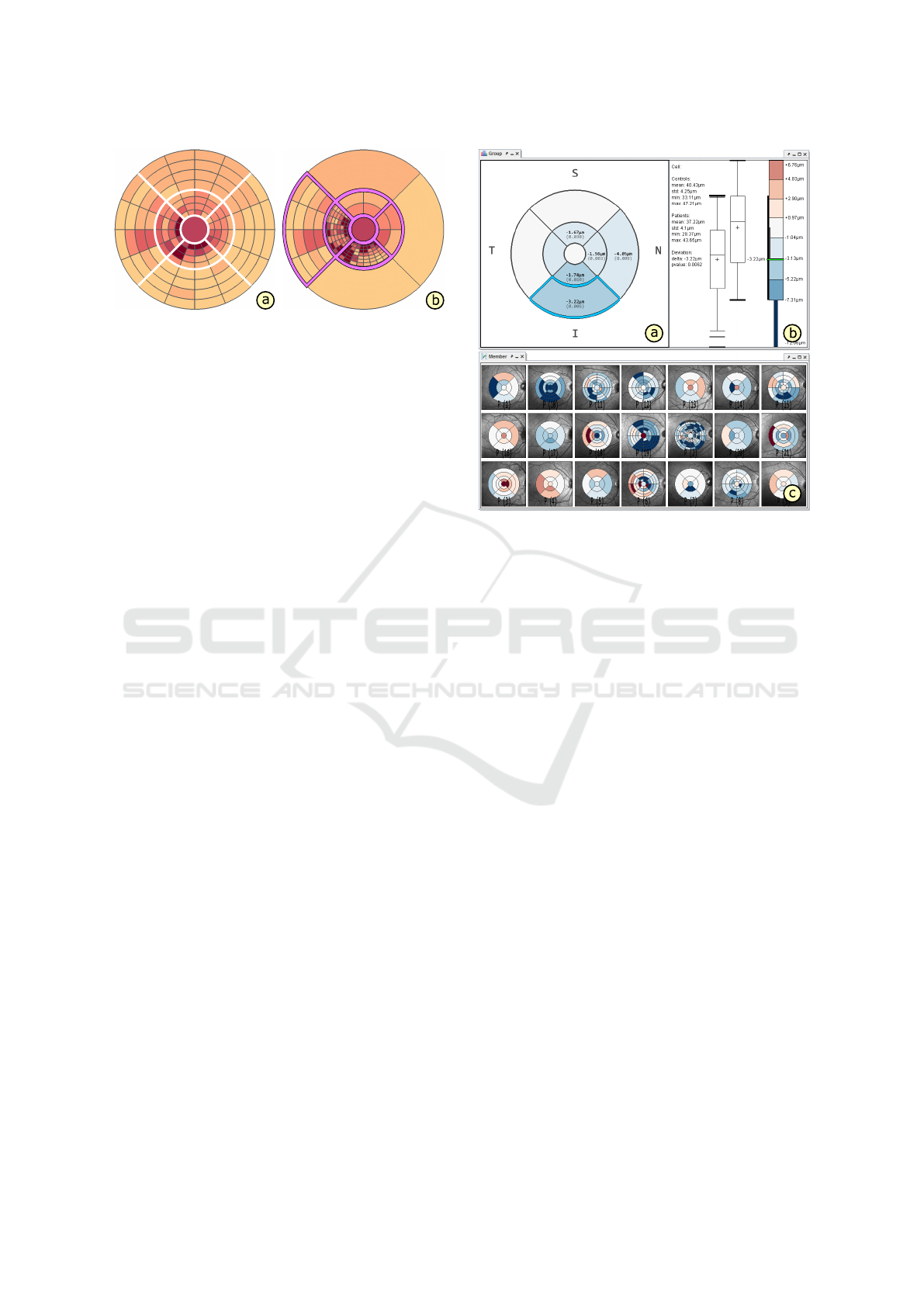
Figure 6: Interactive exploration of grids. The ETDRS grid

layout is marked on a subdivided grid to support the locali-

zation of cells (a). Grid cells with low ratings (purple bor-

ders) are interactively subdivided to investigate details (b).

to be set. This ﬁrst option offers the most freedom

to the expert and allows to obtain a set of grids that

reﬂects speciﬁc needs. The second option is to auto-

matically suggest ﬁtting grids for given thickness data

based on the computed rating and ranking of a prede-

ﬁned set of alternative grid layouts. Such a predeﬁned

set of alternatives may consist of increasingly ﬁner

subdivisions of the ETDRS grid using combinations

of both radial and sector-wise partition strategies. An

expert may further steer the automated selection by

setting additional constraints, e.g, the maximum num-

ber of allowed grid cells. This helps to obtain grids at

an appropriate level of granularity, i.e., grids that cap-

ture even small and localized variations in thickness.

Browsing through grids is supported by interactive

selections from a set of speciﬁed grid layouts. Se-

lected grids are immediately presented in the top-

down view with cells colored and labeled. By ﬂip-

ping through these grids, the data can be explored at

different levels of granularity. For instance, selecting

increasingly ﬁner subdivision of the ETDRS grid al-

lows to analyze the data from overview, i.e., coarsest

grid, to detail, i.e., ﬁnest grid. This helps to under-

stand the data and to localize areas of interest.

Interactively adapting grids allows to reﬁne a se-

lected grid layout. On demand, one or multiple grid

cells may be selected and then merged together or

subdivided by means of the provided partitioning stra-

tegies (cf. Sect. 3.2). This helps to ﬁne-tune grids

for given data based on the expertise of experts. For

instance, while browsing through alternative grids,

a speciﬁc grid is selected, cells are visualized, and

information about the underlying thickness data is

shown. Individual grid cells with low ratings are then

further subdivided to investigate respective areas in

greater detail and the remaining cells are merged to-

gether to provide context information of less relevant

areas. Figure 6b exempliﬁes the adaption of grids.

Comparison of different grids is enabled by juxta-

position of views, explicit encoding of deviations, and

application of statistical tests. The juxtaposition of

Figure 7: Comparison of different grids. The top-down

view (a) and the linked measurement view (b) show a group-

speciﬁc comparison of an aggregated grid of a patient group

to an aggregated grid of a control group. The juxtaposed

small multiple views (c) show an overview of grids of all

individual members of the patient group compared to the

aggregated grid of the control group. Thickness deviations

are explicitly encoded using a diverging color palette.

views supports the comparison of several individual

grids (Fig. 5a, f). In the user interface, multiple in-

stances of the top-down view and measurement view

can be dynamically added and freely arranged. For

a patient-speciﬁc analysis, different grids of the same

patient, e.g., follow-up examinations, or of related pa-

tients, e.g., similar medical cases, can be assigned to

these view instances. Linking the view instances en-

sures that matching parts of the data are shown. For a

group-speciﬁc analysis, individual grids of all mem-

bers of a group are shown as small multiple views

(Fig. 7c). This provides a quick overview and allows

to detect differences between group members.

The explicit encoding of deviations facilitates a di-

rect comparison of a grid to a reference grid. For this

purpose, the coloring of the grid presentation is swit-

ched. The cells are colored using diverging palettes

and by evaluating the stored thickness values with re-

spect to threshold intervals of an aggregated reference

grid. The boundary values vary cell by cell for each

layer, e.g., conﬁdence intervals or percentile bounda-

ries per reference cell. Small deviations from a re-

ference are represented via a light neutral color and

larger negative or positive deviations via respective

darker colors. Displaying deviations helps to evalu-

ate a thickness grid locally in relation to a reference

IVAPP 2019 - 10th International Conference on Information Visualization Theory and Applications

136

grid. Figure 5f and Figure 7a exemplify comparisons

of a grid of a single patient and of an aggregated grid

of an entire patient group to intervals ranging between

the 2.5

and 97.5

percentile boundaries stored in an

aggregated grid of a control group, respectively.

The application of statistical tests allows to quan-

tify the differences between multiple aggregated

grids. For example, for the comparison of aggrega-

ted grids of two different groups, e.g., patients and

controls, an independent two-sample Student’s t-test

is applied and for aggregated grids of more groups an

one-way analysis of variance is performed. The re-

sulting measurements of statistical signiﬁcance, i.e.,

p-values, and effect size are shown as numerical la-

bels. In addition, statistical plots for the cells of each

grid under consideration are shown in the measure-

ment view (Fig. 7b). This illustrates the difference

between the thickness distributions and provides ad-

ditional details about the color-coded deviations in the

comparative grid presentation. Altogether, the functi-

onality eases the evaluation of studies with a lot of

datasets, as this conventionally requires to ﬁrst export

the data of all source grids and then to statistically

analyze them using external software (cf. Sect. 2.2).

5 APPLICATION

We applied and evaluated our research prototype in

cooperation with domain experts. We particularly ai-

med at assessing the utility of our solutions in the con-

text of experimental studies. Here, we brieﬂy describe

one use case, present exemplary results, and reﬂect on

beneﬁts and limitations of our approach.

5.1 Use Case

In this use case, we applied our solutions to study if

early retinal changes in adult patients suffering from

age-related macular degeneration (AMD) can be cap-

tured via different grid representations. In addition,

we were interested in relating the obtained results to

grid representations of healthy control subjects.

A common early sign of AMD is the presence of

drusen in the macula. Drusen are small accumula-

tions of extracellular material that build up between

Bruch’s membrane and the retinal pigment epithelium

(RPE) of the eye (Yoshimura and Hangai, 2014). The

high sensitivity of OCT and the analysis of OCT data

support detecting such small and localized changes,

and hence may contribute to an early diagnosis and

immediate intervention. Yet, in the thickness data of

the RPE, these retinal changes are reﬂected by small

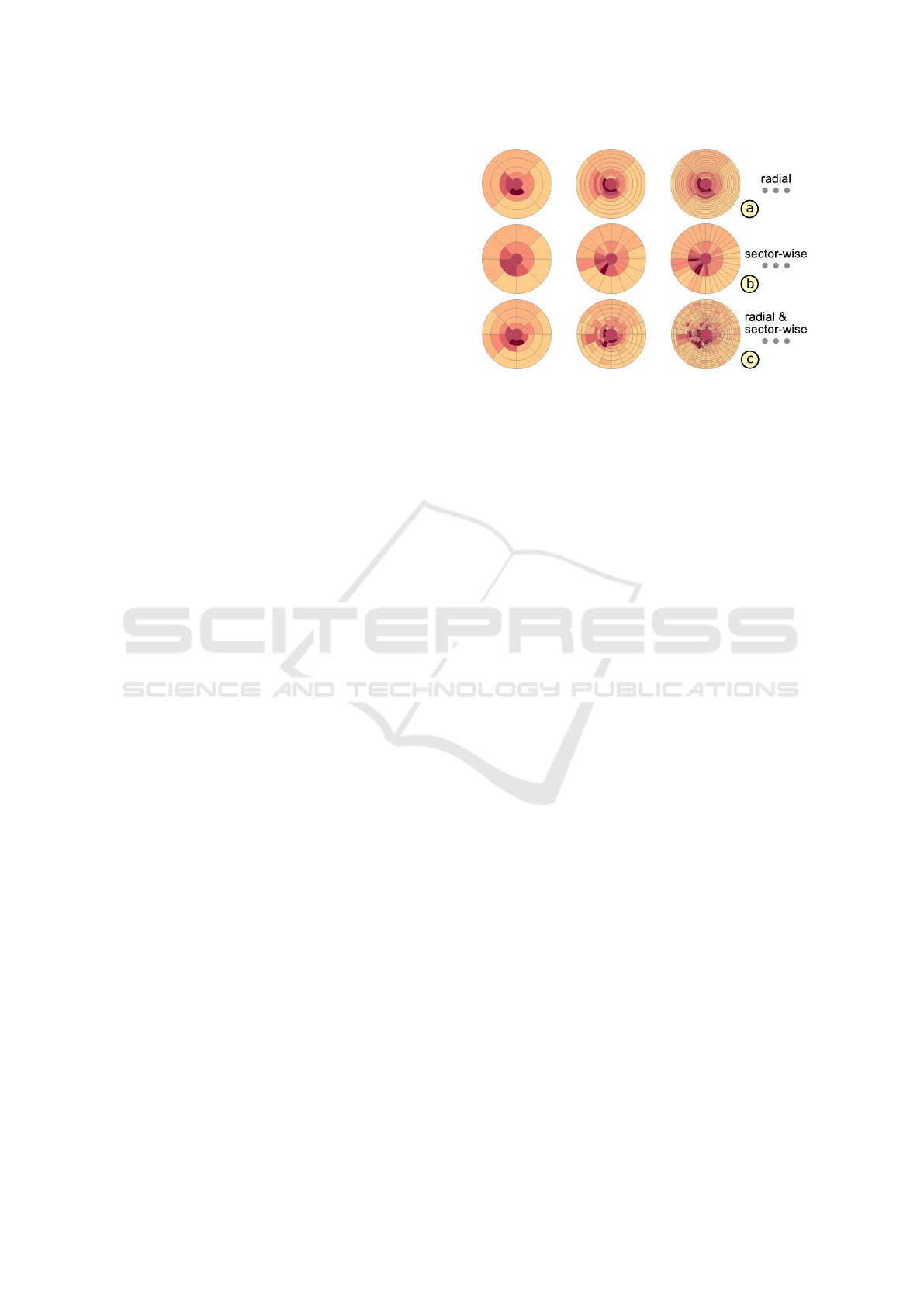
Figure 8: Examples of alternative grids evaluated in our use

case. Three partitioning strategies were applied to derive in-

creasingly ﬁner grids: radial (a), sector-wise (b), and radial

and sector-wise partitions (c).

and localized increases in thickness. We hypothe-

size that conventional ETDRS grids may not always

accurately represent the thickness data in this situa-

tion (cf. Sect. 2.2). In fact, the principal goal of this

study was to assess alternative grids for early retinal

changes in all datasets of participating AMD patients.

The study data were acquired via OCT examinati-

ons of two groups of subjects. The ﬁrst group consists

of 8 adults with AMD and the second group of 20 he-

althy controls. For each subject, the thickness data

of the RPE from one OCT dataset of the macula was

selected for further investigation (28 datasets in total).

Starting from the ETDRS grid, three partitioning stra-

tegies were applied: radial, sector-wise, or radial and

sector-wise partitions. The numbers of radii and sec-

tors were increased in constant steps per strategy up

to a maximum of 129 radii, 256 sectors, and 17 radii

plus 32 sectors respectively. The ﬁnest grid had 513

cells for each strategy. In total, a set of 21 grids, i.e.,

7 grids per strategy, was deﬁned (Fig. 8). In a pre-

process, grid representation were computed and rated

for the thickness data of each dataset in both groups.

The ratings were then summarized per grid to judge

the overall representation quality for each group.

Figure 9 shows an overview of the obtained re-

sults. Note that these results are only meant as a proof

of concept example to demonstrate the feasibility of

our approach. We are aware of the possible bias indu-

ced by the small sample size, which prevents drawing

any medical conclusions. Nonetheless, from a data-

centric perspective, we are able to reason about the

utility of our approach and to summarize our insig-

hts gained from interpreting the results. In this con-

nection, we assume that a superior data representation

is reﬂected by a better rating of grids using the measu-

res introduced in Sect. 3.3, i.e., a good representation

is equal to a low mean standard deviation.

Grid-based Exploration of OCT Thickness Data of Intraretinal Layers

137

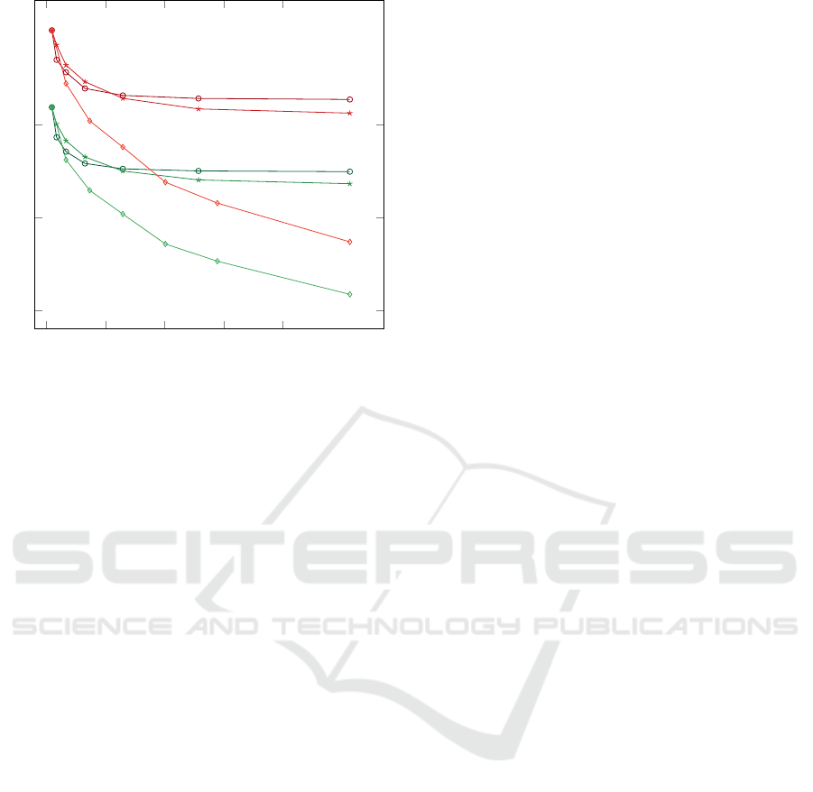
0 100 200 300 400

0.3

0.4

0.5

Cells

Rating

Figure 9: Overview of the study results. The line plot

shows ratings of grids, i.e., summarized standard deviati-

ons, with respect to cell counts. The ratings are depicted for

the thickness data of patients (red) and controls (green) in

relation to three partitioning strategies: radial (a, d), sector-

wise (b, e), and radial and sector-wise (c, f).

In general, all subdivided grids showed better ra-

tings than the ETDRS grid. For the thickness data of

patients, grids based on sector-wise partitions perfor-

med slightly better than grids based on radial partiti-

ons (Fig. 9a, b). Interestingly, for both partition stra-

tegies, an increase in cell count only resulted in better

ratings up to a certain point. In contrast, for combi-

ned radial and sector-wise partitions, an increase in

cell count showed steadily improved ratings (Fig. 9c).

A possible explanation is that early drusen often come

in the form of small, roughly circular-shaped regions

of high thickness. Hence, grid cells that match such

shapes, e.g., cells of grids subdivided via combined

radial and sector-wise partitions, will result in better

overall ratings of respective grids.

For the thickness data of controls, we observed

patterns in the grid ratings that are similar to the re-

sults of patients (Fig. 9d, e, f). This similarity can

probably be explained due to the consideration of pa-

tients with early signs of AMD in the study, i.e., while

the patients’ thickness data showed some noticeable

changes, they were still not too far from the data of

healthy controls. One remarkable difference was, ho-

wever, that the control data generally required fewer

cells to obtain equally good ratings of grids. This is

probably due to the fact that thickness data of healthy

eyes contains less localized variations in thickness.

Thus, an appropriate grid representation of the data

can be achieved with fewer and coarser cells.

5.2 User Feedback and Lessons

Learned

Our solutions are the result of a participatory design

process starting from prior work (R

ohlig et al., 2018).

We cooperated with two groups of domain experts,

including ophthalmic research scientists and a team

of technical and medical professionals from a major

commercial OCT device manufacturer. Throughout

the development, we had close contact with primarily

two ophthalmic experts. Together, we applied and tes-

ted our prototype in collaborative data analysis sessi-

ons using a pair analytics approach (Arias-Hernandez

et al., 2011). We also held repeated demonstration

and feedback sessions with around ten participants of

both expert groups. We jointly identiﬁed challenges

and speciﬁed respective requirements (cf. Sect. 3.1).

Their informal feedback helped us to devise suitable

grid designs and visualization techniques.

During the discussions, the experts stated that they

liked the visual analysis tool because it allowed them

to explore their thickness data at different levels of

granularity. They also appreciated the consideration

of the established ETDRS grid in our grid design.

At the same time, they reassured us that the provi-

ded methods for subdivision, rating, and comparabi-

lity of grids are meaningful enhancements to obtain

appropriate data representations. In fact, the experts

reported that there is a need to ﬁnd grids that match

certain ophthalmic applications, as existing grids are

not always the best choice for their analysis tasks.

In this regard, the results of our experimental

study suggest that our approach can be a useful aid

for identifying appropriate grids for given thickness

data. However, arbitrarily ﬁne subdivided grids are

practically unfeasible for some applications. For ex-

ample, choosing a grid with a large number of cells

may impede further utilization of the data. On this

account, the experts approved to have the rating and

ranking of grids at their disposal. It helped them to de-

cide how much variance they are willing to accept in

a grid with a certain amount of cells. They considered

such decisions to be particularly easy to make in case

of grids that showed only minimally improved ratings

in further subdivision with a certain partitioning stra-

tegy (cf. Fig. 9). Thus, with the provided functiona-

lity, they were able to balance the granularity of grids

and the amount of encoded information.

As another major advantage, the ophthalmic ex-

perts identiﬁed the ability to compare multiple and

possibly differing grids with each other and to the

conventional ETDRS grid. The interlinked top-

down and measurement views helped them to quickly

switch between grids of different layers or datasets

IVAPP 2019 - 10th International Conference on Information Visualization Theory and Applications

138

and to show grid-related details when necessary. For

the analysis of larger studies, they considered the vi-

sualization of deviations between aggregated grids of

groups and the integrated quantiﬁcation of differen-

ces based on statistical tests to be particular useful.

They concluded that reducing the manual analysis ef-

fort and being able to obtain results with higher spatial

accuracy compared to the current analysis procedures

are great beneﬁts.

6 CONCLUSION

We presented an enhanced grid-based data reduction

approach for retinal thickness data. A new grid design

helps to strike a balance between obtaining a compact

data representation and being able to capture more re-

levant information. A coordinated visual analysis tool

supports a grid-based exploration of thickness data at

different levels of granularity. Different grids from

multiple datasets are compared. Alternative grids are

rated and ranked to facilitate the selection of best ﬁt-

ting grids for given thickness data. Our approach con-

stitutes a systematic enhancement of existing work

and hence, provides a ﬁrst step towards supporting

ophthalmologists in their grid-based analysis of intra-

retinal layer thickness.

Our data reduction is based on subdivisions of the

widely-used ETDRS grid layout. This allows to ad-

dress various ophthalmic applications while promo-

ting a more patient-speciﬁc analysis. Beyond taking

the ETDRS grids as a basis, the main ideas of subdivi-

sion, rating, and comparability together with coordi-

nated visualization are applicable to other grid types

as well. This may help to support ﬁne-grained ana-

lyses in more speciﬁc ophthalmic applications, e.g.,

asymmetry analysis of retinal thickness for glaucoma

diagnosis using rectangular grids (Asrani et al., 2011).

During demonstration and feedback sessions, our

experts reported that it is not always known which

grid helps to solve a given analysis task. Hence, re-

search effort exists to ﬁnd new grids that adequately

represent retinal changes of speciﬁc diseases. In this

regard, our rating and ranking of grids may help in

evaluating newly designed grids and sorting out ex-

isting grid types. So far, we used a data-driven ap-

proach to judge the representation quality of grids.

An interesting extension is to also support diagnosis-

driven grid ratings. This requires deﬁning custom me-

asures that match different ophthalmic analysis tasks,

e.g. asymmetry analysis of thickness data. Moreo-

ver, assistance in choosing suitable rating cutoffs for

the selection of grids has to be provided. That way,

automated grid suggestions for speciﬁc tasks or ap-

plication are possible. However, to fully support such

efforts, more work is needed to be able to compare

and rank different grid types.

We ascertained the general utility of our solutions

in ﬁrst tests with domain experts. To improve our de-

sign, we plan further evaluations of our tool in the

context of experimental studies. In this connection, an

interesting open question is how our grid-based analy-

sis approach can be combined with recent map-based

analysis approaches for thickness data of intraretinal

layers, e.g., (R

ohlig et al., 2018). To utilize the be-

neﬁts of both approaches, identifying and evaluating

best practices for each solution is required with re-

spect to an ophthalmic analysis workﬂow.

ACKNOWLEDGEMENTS

This work has been supported by the German Rese-

arch Foundation (project VIES).

REFERENCES

Arias-Hernandez, R., Kaastra, L. T., Green, T. M., and Fis-

her, B. D. (2011). Pair analytics: Capturing reasoning

processes in collaborative visual analytics. In Pro-

ceedings of the Hawaii International Conference on

System Sciences, pages 1–10, Washington, DC, USA.

IEEE Computer Society.

Asrani, S., Rosdahl, J., and Allingham, R. (2011). Novel

software strategy for glaucoma diagnosis: Asymme-

try analysis of retinal thickness. Archives of Ophthal-

mology, 129(9):1205–1211.

Chen, Q., Huang, S., Ma, Q., Lin, H., Pan, M., Liu, X.,

Lu, F., and Shen, M. (2017). Ultra-high resolution

proﬁles of macular intra-retinal layer thicknesses and

associations with visual ﬁeld defects in primary open

angle glaucoma. Scientiﬁc Reports, 7:41100.

Chew, E., Klein, M., Ferris, F., Remaley, N., Murphy, R.,

Chantry, K., Hoogwerf, B., and Miller, D. (1996). As-

sociation of elevated serum lipid levels with retinal

hard exudate in diabetic retinopathy: Early treatment

diabetic retinopathy study (ETDRS) report 22. Archi-

ves of Ophthalmology, 114(9):1079–1084.

Garrido, M. G., Beck, S. C., M

uhlfriedel, R., Julien, S.,

Schraermeyer, U., and Seeliger, M. W. (2014). To-

wards a quantitative OCT image analysis. PLOS ONE,

9(6):1–10.

Garvin, M. K., Abramoff, M. D., Wu, X., Russell, S. R.,

Burns, T. L., and Sonka, M. (2009). Automated 3-

D intraretinal layer segmentation of macular spectral-

domain optical coherence tomography images. IEEE

Transactions on Medical Imaging, 28(9):1436–1447.

Glittenberg, C., Krebs, I., Falkner-Radler, C., Zeiler, F.,

Haas, P., Hagen, S., and Binder, S. (2009). Advan-

tages of using a ray-traced, three-dimensional rende-

ring system for spectral domain cirrus HD-OCT to vi-

Grid-based Exploration of OCT Thickness Data of Intraretinal Layers

139

sualize subtle structures of the vitreoretinal interface.

Ophthalmic Surgery Lasers and Imaging, 40(2):127–

134.

otze, A., von Keyserlingk, S., Peschel, S., Jacoby, U.,

Schreiver, C., K

ohler, B., Allgeier, S., Winter, K.,

ohlig, M., J

unemann, A., Guthoff, R., Stachs, O.,

and Fischer, D.-C. (2018). The corneal subbasal nerve

plexus and thickness of the retinal layers in pediatric

type 1 diabetes and matched controls. Scientiﬁc Re-

ports, 8(1).

Harrower, M. and Brewer, C. A. (2003). Colorbrewer.org:

An online tool for selecting colour schemes for maps.

The Cartographic Journal, 40(1):27–37.

Mayer, M. A., Hornegger, J., Mardin, C. Y., and Tornow,

R. P. (2010). Retinal nerve ﬁber layer segmentation

on FD-OCT scans of normal subjects and glaucoma

patients. Biomedical Optics Express, 1(5):13581383.

Mazzaferri, J., Beaton, L., Hounye, G., N. Sayah, D., and

Costantino, S. (2017). Open-source algorithm for au-

tomatic choroid segmentation of OCT volume recon-

structions. Scientiﬁc Reports, 7.

ohlig, M., Schmidt, C., Prakasam, R. K., Schumann, H.,

and Stachs, O. (2018). Visual analysis of retinal chan-

ges with optical coherence tomography. The Visual

Computer, 34(9):1209–1224.

Schindelin, J., Rueden, C. T., Hiner, M. C., and Eliceiri,

K. W. (2015). The ImageJ ecosystem: An open plat-

form for biomedical image analysis. Molecular Re-

production and Development, 82(7-8):518–529.

Yoshimura, N. and Hangai, M. (2014). OCT Atlas. Sprin-

ger, Berlin, Germany.

IVAPP 2019 - 10th International Conference on Information Visualization Theory and Applications

140