
Efficient Imputation Method for Missing Data Focusing on
Local Space Formed by Hyper-Rectangle Descriptors
Do Gyun Kim and Jin Young Choi
Department of Industrial Engineering, Ajou University, Suwon, Korea
{rlaehrbs90, choijy}@ ajou.ac.kr
Keywords: Missing Data, Imputation, Hyper-Rectangle Descriptor, Local Space.
Abstract: In real world data set, there might be missing data due to various reasons. These missing values should be
handled since most data analysis methods are assuming that data set is complete. Data deletion method can
be simple alternative, but it is not suitable for data set with many missing values and may be lack of
representativeness. Furthermore, existing data imputation methods are usually ignoring the importance of
local space around missing values which may influence quality of imputed values. Based on these
observations, we suggest an imputation method using Hyper-Rectangle Descriptor () which can focus
on local space around missing values. We describe how data imputation can be carried out by using ,
named _, and validate the performance of proposed imputation method with a numerical
experiment by comparing to imputation results without . Also, as a future work, we depict some ideas
for further development of our work.
1 INTRODUCTION
Some data might be missing during collection due to
various reasons such as physical or logical errors.
However, since most of data analysis techniques
cannot be performed properly with missing data,
handling missing data is very important in machine
learning area. As an alternative, one can simply
exclude data with missing parts and analyze the rest
of fully collected data, which is called data deletion
method (McKnight et al., 2007). This approach can
perform well only if few data points are missing.
However, in real world data, there can be many
missing data points, and analysis results obtained
from using only fully known data cannot represent
the whole data set. Therefore, we need a data
imputation method that replaces missing data with
new values estimated from fully collected data,
rather than excluding them. In this case, although
imputed values are estimated from observed data,
scalability of original data set can be preserved, and
data analysis can be applied to it that is a complete
data set.
Generally, in data imputation process, local
space around missing data is important since
behavior of missing data is more likely to follow
data pattern in local space rather than whole feature
space. However, although there are many researches
about missing data imputation, there exist few
approaches focusing on local space. Some
imputation methods including -Nearest Neighbors
(-NN) utilizes information of local space. However,
they have their own limitations such as parameter
selection and ambiguous standard definition of local
space.
Based on these observations, we propose an
efficient imputation method that can (i) define local
space around missing data systematically and (ii)
impute missing values by focusing on that local
space. Specifically, we suggest _ as a
missing data imputation method using Hyper-
Rectangle Descriptor ( ) that was originally
developed to carry out one-class classification
(Jeong et al., 2019). The basic idea of is to
divide feature space into Hyper-Rectangles (H-
RTGLs), formed by geometric rules called intervals,
and classify instances in H-RTGLs as target class.
Therefore, H-RTGLs as can be considered as a
certain local space including some instances and can
be used to overcome one of limitations of existing
missing data imputation methods.
The rest of this paper is organized as follows.
Section 2 describes the literature survey about
existing missing data imputation methods. We
suggest details of the suggested -based
imputation method in Section 3. Then, we validate
Kim, D. and Choi, J.
Efficient Imputation Method for Missing Data Focusing on Local Space Formed by Hyper-Rectangle Descriptors.
DOI: 10.5220/0007582104670472
In Proceedings of the 8th International Conference on Operations Research and Enterprise Systems (ICORES 2019), pages 467-472
ISBN: 978-989-758-352-0
Copyright
c
2019 by SCITEPRESS – Science and Technology Publications, Lda. All rights reserved
467

the performance of proposed method by a numerical
experiment in Section 4. Finally, we conclude our
work and pose some ideas for future works in
Section 5.
2 RELATED WORKS
There exist many imputation methods to handle
missing data these days. For example, all missing
data can be replaced with a single value. One can
also consider using basic machine learning
techniques such as regression analysis, -NN and
decision tree, and so on.
Mean or median imputation is a representative
single value imputation method, which imputes
missing values using a mean or median of
observations not missing (Little and Rubin, 2014).
Such imputation method is easy to implement and
can perform well if there are few missing values.
However, imputation with single value such as mean
or median is not suitable in most cases since it
cannot reflect variance and distribution of data, and
imputed values are lack of representativeness.
By regression, one can obtain a mathematical
model that describes relationship of input and output
variables. Data imputation with regression is
performed as follows: At first, a regression model is
formed by using a feature with missing value as
output variable and other features as input variables.
Then, missing value of the feature can be computed
by observed values of other features (Brown and
Kros, 2003). Data imputation methods using
regression can be categorized according to the
method to formulate regression model. Regression
model using Least-Squares (LS) is most common
and basic (Raghunathan et al., 2001). Based on this,
calculating LS sequentially or iteratively was also
considered (Zhang et al., 2008; Shi et al., 2013).
More complicated regression model such as Support
Vector Regression (SVR) and nonlinear regression
were also tackled (Aydilek and Arslan, 2013; Tang
and Zhao, 2013). Clear disadvantage of regression-
based imputation methods is that they cannot focus
on local relationship.
Data imputation using -NN utilizes information
about the nearest neighbors of missing data.
Specifically, -NN imputation replaces missing
values as follows. We select nearest neighbors by
considering features not in missing data. Then,
missing value is estimated from features of observed
nearest neighbors by using means or weighted
means and so on (Chen and Shao, 2000). Choosing
nearest neighbors sequentially or iteratively is one of
the most common variations of -NN-based
imputation (Zhang, 2012; Kim et al., 2004). Huang
and Zhu (2002) proposed imputation method based
on pseudo-nearest neighbors, expected to follow the
same Gaussian distribution. Christobel and
Sivaprakasam (2013) devised class-wise -NN that
utilizes class information to choose nearest
neighbors for labelled data set. García-Laencina et
al., (2009) adopted mutual information as distance
metrics for choosing nearest neighbor. Jonsson and
Wohlin (2004) evaluated the performance of various
-NN-based imputation methods. -NN-based
imputation methods could partially utilize local
relationship. However, there was no implicit
standard about how to decide .
Other methods suggested for missing data
imputation including decision tree are as follows. To
impute missing data, decision tree can be generated
by rules to calculate missing value. C4.5 and CN2
are representative algorithms to build decision tree
(Grzymala-Busse and Hu, 2000; Batista and Monard,
2003). Decision tree is useful to impute missing data
by intuitive rules, but it may become too complex in
case of using many features not scalable well. Also,
it can be over fitted easily. Expectation-
Maximization (EM) algorithm tries to impute
missing data with new values likely to be missing,
while maximizing likelihood function (Gold and
Bentler, 2000). It can find imputation values
systematically, but its performance depends on
initial parameter setting. Furthermore, Bertsimas et
al. (2017) considered missing data imputation as an
optimization problem and proposed fast first-order
methods to obtain high quality solutions for it.
3 SUGGESTION OF NEW
IMPUTATION METHOD
3.1 Problem Definition and Solution
Framework
We define notation and index necessary for
describing missing data imputation problem as
follows. We assume a whole data set
x
,x
,…, x
, containing data points. Then, -th
instance x
1,2,…, can be expressed as x
,
,…,
, where is the total number of
features. Also, there is an index set of missing
entries ,| -th feature of -th instance is
missing. As a result, the objective of imputation
problem is to substitute missing entry
,,∈
by using fully collected data points.
ICORES 2019 - 8th International Conference on Operations Research and Enterprise Systems
468
Meanwhile, we carry out the imputation of
missing data by using
, which is a method
generating based on interval merging. The
framework of _ tackled in this research
can be depicted as Figure 1. At first, we obtain
from data points except for missing ones and
fit a linear regression model for each resulted
.
Then, we identify
expected to include
missing data and impute missing value from
regression model fitted into
. Subsection 3.2
describes detailed procedure of missing data
imputation method by using
.
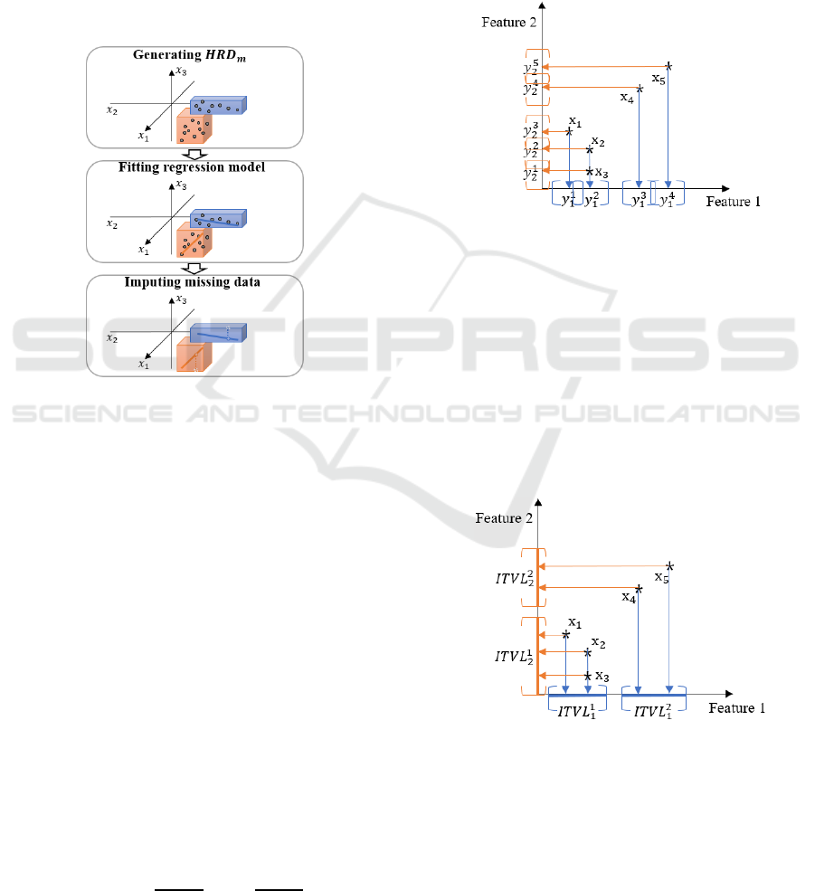
Figure 1: Framework of imputation USING
.
3.2 Detailed Procedure of
_ using
At first, we generate
from fully collected data
points as follows (Jeong et al., 2018). The first step
to construct
is to generate intervals for each
feature , which is main component of generating
hyper-rectangle. An interval is calculated from a set
of projection points of all instances into feature .
Specifically, we define the projection point of
instance x
into feature as
x
,∀.
(1)
By using (1), we can obtain the set of projection
points
containing
points as
,
,…,
,
(2)
where
is -th smallest value in
satisfying
⋯
. For each projection point
, we
define an interval
as
2
,
2
,∀
,
(3)
where
is interval length calculated by the
number of projection points with the same value and
some parameters. Since intervals
are
generated considering all projection points
, there
can be overlapped intervals. For example, Figure 2
is an example of interval generation in two-
dimensional feature space with five instances
x
,x
,x
,x
,x
. All instances were projected to
each feature, and intervals were generated from each
of projection points.
Figure 2: An example of interval generation for
.
While calculating intervals from projection
points, some intervals may be overlapped. These
overlapped intervals are merged, which is resulted in
a set of disjoint intervals containing
disjoint
intervals as
,
,…,
. For
example, there are overlapped intervals in Figure 2
such as
and
. After applying
merging operation to all of these overlapped
intervals, resulting disjoint intervals in above-
mentioned example were depicted in Figure 3.
Figure 3: Disjoint intervals resulted from merging.
Next step is to get conjunction of these disjoint
intervals. Conjunction of intervals can be obtained
by cartesian product of intervals generated from all
features. However, some conjunction of intervals
may not include any instance since intervals are
generated feature by feature. For example,
conjunction of
and
does not include
Efficient Imputation Method for Missing Data Focusing on Local Space Formed by Hyper-Rectangle Descriptors
469
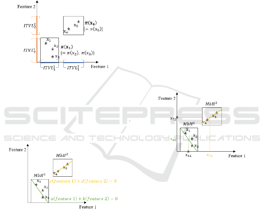
any instance. Thus, interval conjunction should be
defined by considering instances. Specifically,
interval conjunction
x
including instance x
is
expressed as
x
⋀
⋀…⋀
,∀,
(4)
where
x
∈
,∀. From the information
of disjoint intervals in Figure 3, for example, two
interval conjunctions can be drawn as Figure 4.
Figure 4: Interval conjunctions obtained from instances.
Merging-based H-RTGLs, , are constructed
by adjusting volume of each interval conjunction.
However, some may be overlapped even if
they are formulated from disjoint intervals. We
recommend Jeong et al., (2018) for revealing
detailed adjusting procedure or other contents
including roles of parameters.
Figure 5: Two regression models fitted into two s.
After such are formulated, instances can
be classified by
s. In other words, local spaces
expected to include each instance with missing
feature are identified, and imputation of missing data
can be carried out by considering such relationship.
We fit into a linear regression model for each ,
and the regression model is calculated considering
only instances belonging to . Since there exist
two s in above-mentioned example, two linear
regression models can be fitted into as depicted in
Figure 5.
Then, missing data can be imputed by using
resulted linear regression model. Suppose that there
are two more instances with missing entries x
and
x
, which are not used to formulate due to
missing entries. In addition, the index set of missing
entries is given as
6,2
,
7,1
, which
means feature 2 of x
and feature 1 of x
are missing.
If known values of x
(
) and x
(
) are
belonging to respective , imputed values should
be calculated from the corresponding linear
regression model. Figure 6 shows the imputation
procedure for the given example. Missing values of
instance x
(
) and instance x
(
) are imputed
from the corresponding regression models. If there
exist two or more candidates of , one is
randomly selected. The probability of each to
be selected is given by the number of instances
belonging to . If there is no to be selected,
the nearest is used instead. In case of two or
more missing features exits in one instance,
candidate is selected at first, and then random
value on regression model corresponding to is
chosen as an imputation value.
Figure 6: Imputed values for missing data.
4 A NUMERICAL EXPERIMENT
4.1 Experimental Design
To validate the performance of proposed missing
data imputation method, we committed a numerical
experiment by using real world dataset from UCI
machine learning repository. We considered three
datasets named Iris, Wine, E.coli. The number of
instances and features
,
in each dataset is
150,4
,
173,13
,
284,7
, respectively. Missing
entries are randomly generated in dataset at Missing
at Completely Random (MCAR), and we used three
missing percentage from 10% to 20%. We
implemented two versions of _ with
different parameter configurations, represented by
_
and _
. The former
ICORES 2019 - 8th International Conference on Operations Research and Enterprise Systems
470

approach generates s from longer intervals,
which make size of to increase. In other words,
_
separates whole feature space
densely with many small s. Also, we
considered regression model fitted without
as
control group. To evaluate imputation performance,
we calculated Mean Absolute Percentage Error
(MAPE) defined as
100%
, (5)
where
is the actual value, and
is the forecasted
value.
4.2 Experimental Results
Tables 1 to 3 summarize imputation performance of
_ and control group in three datasets. 10
iterations were committed with the same missing
percentage in dataset.
Table 1: Experimental result from Iris data.
Missing percentage
10% 15% 20%
Avg. MAPE (standard deviation)
_
(,)= (8,0.5)
9.3 (1.2) 13.9 (1.4) 18.2 (1.3)
_
(,)= (2,0.2)
8.2 (0.9) 11.3 (1.0) 17.4 (1.2)
Regression 13.2 (1.8) 19.4 (2.5) 26.8 (2.6)
Table 2: Experimental result from Wine data.
Missing percentage
10% 15% 20%
Avg. MAPE (standard deviation)
_
(,)= (8,0.5)
10.2 (1.3) 13.3 (0.9) 18.7 (2.9)
_
(,)= (2,0.2)
11.9 (0.8) 13.8 (1.4) 20.2 (2.3)
Regression 16.2 (1.3) 19.3 (2.1) 28.3 (3.2)
Table 3: Experimental result from e.coli data.
Missing percentage
10% 15% 20%
Avg. MAPE (standard deviation)
_
(,)= (8,0.5)
13.5 (1.6) 17.9 (1.3) 21.4 (1.9)
_
(,)= (2,0.2)
13.7 (1.8) 16.8 (2.1) 20.4 (2.2)
Regression 15.9 (1.1) 20.3 (2.2) 27.9 (3.1)
As a result, imputation performance of
_ was better than simple regression.
This means that utilizing information of local space
and local relationship can improve imputation
performance of missing data. Regarding comparison
of _
and _
, slight
dominance of _
was observed in Iris
dataset, while imputation performance of
_
was a little bit better in Wine dataset.
From these results, we can infer that dominance of
different _ methods might depend on
dataset.
5 CONCLUSIONS
In this paper, we proposed a new imputation method
for missing data that can replace missing values by
focusing local space having high potential to include
missing data. Especially, _ proposed in
this paper enabled local spaces to be identified
systematically. _ was implemented by
segmenting feature space into H-RTGLs and fitting
regression models, which was a basis for imputation
of missing values. As a result, missing values could
be imputed by utilizing information of local space
by using _ .
Even if performance of _ was
validated through a numerical experiment, there are
still plenty of further works to consider. Most of all,
result of _ should be compared to other
imputation methods rather than simple regression.
Also, imputation performance may be improved by
tuning parameters of
, since generation of
is sensitive to these parameters. Thus,
thorough research of parameter tuning can be
considered. We also plan to apply _ for
large or complex dataset to verify scalability or
generality of it. Moreover,
and imputation
with regression can be substituted by other methods
that have the same role. Detailed policies for
multiple missing attributes in one instance can be
another future research area.
ACKNOWLEDGEMENTS
This work was supported by the National Research
Foundation of Korea (NRF) grant funded by the
Korea government (MSIT) (No. NRF-
2017R1A2B4009841).
REFERENCES
Aydilek, I. B., & Arslan, A. (2013). A hybrid method for
imputation of missing values using optimized fuzzy c-
Efficient Imputation Method for Missing Data Focusing on Local Space Formed by Hyper-Rectangle Descriptors
471

means with support vector regression and a genetic
algorithm. Information Sciences, 233, 25-35.
Batista, G. E., & Monard, M. C. (2003). An analysis of
four missing data treatment methods for supervised
learning. Applied artificial intelligence, 17(5-6), 519-
533.
Bertsimas, D., Pawlowski, C., & Zhuo, Y. D. (2017).
From predictive methods to missing data imputation:
An optimization approach. The Journal of Machine
Learning Research, 18(1), 7133-7171.
Brown, M. L., & Kros, J. F. (2003). Data mining and the
impact of missing data. Industrial Management &
Data Systems, 103(8), 611-621.
Chen, J., & Shao, J. (2000). Nearest neighbor imputation
for survey data. Journal of Official statistics, 16(2),
113.
Christobel, Y. A., & Sivaprakasam, P. (2013). A New
Classwise k Nearest Neighbor (CKNN) method for the
classification of diabetes dataset. International Journal
of Engineering and Advanced Technology, 2(3), 396-
400.
García-Laencina, P. J., Sancho-Gómez, J. L., Figueiras-
Vidal, A. R., & Verleysen, M. (2009). K nearest
neighbours with mutual information for simultaneous
classification and missing data imputation.
Neurocomputing, 72(7-9), 1483-1493.
Gold, M. S., & Bentler, P. M. (2000). Treatments of
missing data: A Monte Carlo comparison of RBHDI,
iterative stochastic regression imputation, and
expectation-maximization. Structural Equation
Modeling, 7(3), 319-355.
Grzymala-Busse, J. W., & Hu, M. (2000, October). A
comparison of several approaches to missing attribute
values in data mining. In International Conference on
Rough Sets and Current Trends in Computing. 378-
385
Huang, X., & Zhu, Q. (2002). A pseudo-nearest-neighbor
approach for missing data recovery on Gaussian
random data sets. Pattern Recognition Letters, 23(13),
1613-1622.
Jeong, I., Kim, D. G., Choi, J. Y., & Ko, J. (2019).
Geometric one-class classifiers using hyper-rectangles
for knowledge extraction. Expert Systems with
Applications, 117, 112-124.
Jonsson, P., & Wohlin, C. (2004, September). An
evaluation of k-nearest neighbour imputation using
likert data. In Software Metrics, 2004. Proceedings.
10th International Symposium on. 108-118
Kim, K. Y., Kim, B. J., & Yi, G. S. (2004). Reuse of
imputed data in microarray analysis increases
imputation efficiency. BMC bioinformatics, 5(1), 160.
Little, R. J., & Rubin, D. B. (2014). Statistical analysis
with missing data. John Wiley & Sons.
McKnight, P. E., McKnight, K. M., Sidani, S., &
Figueredo, A. J. (2007). Missing data: A gentle
introduction. Guilford Press.
Shi, F., Zhang, D., Chen, J., & Karimi, H. R. (2013).
Missing value estimation for microarray data by
Bayesian principal component analysis and iterative
local least squares. Mathematical Problems in
Engineering 2013, 1-5.
Tang, N. S., & Zhao, P. Y. (2013). Empirical likelihood-
based inference in nonlinear regression models with
missing responses at random. Statistics, 47(6), 1141-
1159.
Templ, M., Kowarik, A., & Filzmoser, P. (2011). Iterative
stepwise regression imputation using standard and
robust methods. Computational Statistics & Data
Analysis, 55(10), 2793-2806.
Trivellore E Raghunathan, James M Lepkowski, John Van
Hoewyk, and Peter Solenberger. A multivariate
technique for multiply imputing missing values using
a sequence of regression models. Survey Methodology,
27(1):85-96, 2001
Tutz, G., & Ramzan, S. (2015). Improved methods for the
imputation of missing data by nearest neighbor
methods. Computational Statistics & Data Analysis,
90, 84-99.
Zhang, S. (2012). Nearest neighbor selection for
iteratively kNN imputation. Journal of Systems and
Software, 85(11), 2541-2552.
Zhang, X., Song, X., Wang, H., & Zhang, H. (2008).
Sequential local least squares imputation estimating
missing value of microarray data. Computers in
biology and medicine, 38(10), 1112-1120.
ICORES 2019 - 8th International Conference on Operations Research and Enterprise Systems
472
