Analyzing the Linear and Nonlinear Transformations of AlexNet to Gain
Insight into Its Performance
Jyoti Nigam, Srishti Barahpuriya and Renu M. Rameshan
Indian Institute of Technology, Mandi, Himachal Pradesh, India
Keywords:
Convolution, Correlation, Linear Transformation, Nonlinear Transformation.
Abstract:
AlexNet, one of the earliest and successful deep learning networks, has given great performance in image clas-
sification task. There are some fundamental properties for good classification such as: the network preserves
the important information of the input data; the network is able to see differently, points from different classes.
In this work we experimentally verify that these core properties are followed by the AlexNet architecture. We
analyze the effect of linear and nonlinear transformations on input data across the layers. The convolution fil-
ters are modeled as linear transformations. The verified results motivate to draw conclusions on the desirable
properties of transformation matrix that aid in better classification.
1 INTRODUCTION AND
RELATED WORK
Convolutional neural networks (CNNs) have led to
considerable improvements in performance for many
computer vision (LeCun et al., 1989; Krizhevsky
et al., 2012) and natural language processing tasks
(Young et al., 2018). In recent literature there are
many papers (Giryes et al., 2016; Sokoli
´
c et al., 2017;
Sokoli
´
c et al., 2017; Oyallon, 2017) which provide an
analysis on why deep neural networks (DNNs) are ef-
ficient classifiers. (Kobayashi, 2018; Dosovitskiy and
Brox, 2016) provide an analysis of CNNs by looking
at the visualization of the neuron activations. Statis-
tical models (Xie et al., 2016) have also been used to
derive feature representation based on a simple statis-
tical model.
We choose to analyze the network in a method dif-
ferent from all the above by modeling the filters as a
linear transformation. The effect of nonlinear opera-
tions is analyzed by using measures like Mahalanobis
distance and angular as well as Euclidean separation
between points of different classes.
AlexNet (Krizhevsky et al., 2012) is one of the
oldest successful CNNs that recognizes images of the
ImageNet dataset (Deng et al., 2009). We analyze ex-
perimentally this network with an aim of understand-
ing the mathematical reasons for its success. We use
data from two classes of ImageNet to study the per-
formance of AlexNet.
The contributions of this analysis are as follows:
• We derive the structure of the linear transforma-
tion corresponding to the convolution filters and
analyze its effect on the data using the bounds on
the norm of the linear transformation.
• Using a specific data selection plan we show em-
pirically that the data from the same class shrinks
and separation increases between two different
classes.
2 ANALYSIS
AlexNet employs five convolution layers and three
max pooling layers for extracting features. Further-
more, the three fully connected layers for classifying
images as shown in Fig.1. Each layer makes use of
the rectified linear unit (ReLU) for nonlinear neuron
activation.
In CNNs, feature extraction from the input data
is done by convolution layers while fully connected
layers perform as classifiers. Each convolution layer
generates a feature map that is in 3D tensor format and
fed into the subsequent layer. The feature map from
the last convolution layer is given to fully connected
layers in the form of a flattened vector and a 1000 di-
mensional vector is generated as output of fully con-
nected layer. This is followed by normalization and
then a softmax layer is applied. In the normalized out-
put vector, each dimension refers to the probability of
the image being the element of each image class.
860
Nigam, J., Barahpuriya, S. and Rameshan, R.
Analyzing the Linear and Nonlinear Transformations of AlexNet to Gain Insight into Its Performance.
DOI: 10.5220/0007582408600865
In Proceedings of the 8th International Conference on Pattern Recognition Applications and Methods (ICPRAM 2019), pages 860-865
ISBN: 978-989-758-351-3
Copyright
c
 2019 by SCITEPRESS – Science and Technology Publications, Lda. All rights reserved

Figure 1: AlexNet Architecture (Kim et al., 2017).
CNN has more than one linear transformations
and two types of nonlinear transformations (ReLU
and pooling) which are used in repetition. The the
nonlinear transformation confines the data to the pos-
itive orthant of higher dimension.
2.1 Analysis of Linear Transformation
The main operation in CNNs is convolution. The fil-
ters are correlated with the input to get feature maps
and this operation is termed as convolution in the liter-
ature. Since correlation is nothing other than convolu-
tion without flipping the kernel, correlation operation
can also be represented as a matrix vector product.
We refer to this matrix as the linear transformation.
1D and 2D correlation can be represented as shown in
Eq. (1) and Eq. (2), respectively.
y(n) =
∑
k
h(k)x(n + k), (1)
y(m,n) =
∑
l
∑
k
h(l, k)x(m + l,n + k), (2)
where x is the input and y is the output and h is the
kernel. Eq.1 leads to a Toeplitz matrix and Eq.2 leads
to a block Toeplitz matrix. In CNNs notice that the or-
der of convolution is higher and correspondingly one
gets a matrix which is Toeplitz with Toeplitz blocks.
Typically each layer has multiple filters leading to
multiple maps and the Toeplitz matrix corresponding
to each filter is stacked vertically to get the overall
transformation from the input space to output space.
As an example let x ∈ R
N
1
×N
2
×N
3
be an input vec-
tor and y ∈ R
M
1
×M
2
×M
3
be the output vector, where
N
3
and M
3
are number of channels in input and num-
ber of filters, respectively. Then the transformation
matrix T is such that T ∈ R
M
1
M
2
M
3
×N
1
N
2
N
3
. T is ob-
tained by stacking f
k
, where 1 ≤ k ≤ M
3
, as shown
in Fig.2. Each f
k
is Toeplitz with Toeplitz blocks and
Figure 2: Convolution operation. The input is of size
N
1
N
2
N
3
×1 and there are M
3
filters ( f
1
,..., f
M
3
) which gen-
erate M
3
feature maps (m
1
,...,m
M
3
).
has full rank. The input x is convolved with each filter
generating a feature map m
k
. Eq.(3) gives the descrip-
tion of convolution operation.
y = T x. (3)
2.1.1 Analysis based on Nature of
Transformation Matrix
The desirable properties for transformation matrix (T )
to aid classification are:
1. The null space of T should be such that the differ-
ence of vectors from two different classes should
not be in the null space of T. This in turn demands
that the difference should not lie in null space of
f
k
, 1 ≤ k ≤ M
3
, i.e. if x
i
∈ C
i
and x
j
∈ C
j
, where
C
i
and C
j
are different classes,
x
j
− x
i
/∈ N ( f
k
), 1 ≤ k ≤ N. (4)
Proof. Let x
1
,x
2
∈ R
N
1
×N
2
×N
3
be two points and
their difference x = x
1
− x
2
, the norm of x is,
kxk= kx
2
− x
1
k. (5)
x
1
,x
2
are transformed to
y
1
= T x
1
, y
2
= T x
2
. (6)
Analyzing the Linear and Nonlinear Transformations of AlexNet to Gain Insight into Its Performance
861

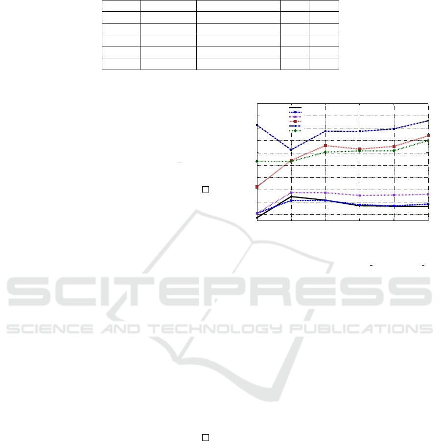
Table 1: Analysis of norm values at each layer.
Layers Total filters Filters: k T k
2
< 1 Min Max
1 96 13 0.28 4.16
2 256 2 0.03 4.26
3 384 2 0.96 2.22
4 384 6 0.96 2.12
5 256 0 1.16 2.19
Norm of the difference of y
1
and y
2
is
ky
2
− y
1
k= kT (x
2
− x
1
)k, (7)
That can be written as:
kT (x
2
− x
1
)k= (
M
3
∑
k=1
k f
k
(x
2
− x
1
)k
2
)
1
2
,
x
2
−x
1
/∈ N (T ) only if x
2
−x
1
/∈ N ( f
k
) ∀k. This is
important to maintain separation between classes
after the transformation.
2. λ
min
(T T
T
) > 1, λ
max
(T T
T
) > 1, where λ
min
and
λ
max
are the minimum and maximum eigenvalues,
respectively of T T
T
.
Proof. For proper classification, two vectors from
different classes should be separated at least by
kx
2
− x
1
k. Since
y
2
− y
1
= T (x
2
− x
1
),
ky
2
− y
1
k = kT (x
2
− x
1
)k,
= k(x
2
− x
1
)kkT zk, wherekzk= 1.
Let λ
min
and λ
max
are the minimum and max-
imum eigenvalues, respectively of T T
T
, then
λ
min
≤ kT zk≤ λ
max
, and hence
λ
min
k(x
2
− x
1
)k≤ k(y
2
− y
1
)k≤ λ
max
k(x
2
− x
1
)k.
(8)
From Eq.(8) it is evident that λ
min
,λ
max
> 1 is
ideal. We observe that for all the layers λ
min
> 0
as shown in Tab. 1 but λ
min
> 1 only for the last
layer . Note that it is not necessary that when all
full rank f
k
s are vertically stacked the T is full
rank, but we observe from the experiments that it
is full rank.
2.2 Analysis of Nonlinear
Transformation
In this section, we analyze and verify (using AlexNet
and its pre-trained weights) the effect of nonlinear
10
20
30
40
50
60
70
80
90
100
0 1 2 3 4 5
Angles
Layers
Angles between representative points of both classes
Near_Min
Medium_Min
Far_Min
Near_Max
Medium_Max
Far_Max
Figure 3: Angles between representative points of both the
classes. The first entry in x−axis shows the input value fol-
lowed by five layers of AlexNet. Near min and Near max
are minimum and maximum angle values, respectively from
the near region. Similarly for medium and far regions the
minimum and maximum values are shown.
transformations on the input data. In this direction
there is a work (Giryes et al., 2016), which provides
a study about how the distance and the angle changes
after the transformation within the layers. The anal-
ysis in (Giryes et al., 2016) is based on the networks
with random Gaussian weights and it exploits tools
used in the compressed sensing and dictionary learn-
ing literature. They showed that if the angle between
the inputs is large then the Euclidean distance be-
tween them at the output layer will be large and vice-
versa.
We analyze the effect of nonlinear transformations
on the input data by measuring the following key-
points. The details are given in the experiments sec-
tion.
• Effect of transformation on angles between repre-
sentative points of two classes
• Transformation in Euclidean distance of points
from mean within each class.
• Mahalanobis distance between the mean points of
two classes.
• Minimum and maximum Euclidean distance
among points within class and between class.
ICPRAM 2019 - 8th International Conference on Pattern Recognition Applications and Methods
862

3 EXPERIMENTS
In this section we analyze how the angles and Eu-
clidean distances change within the layers. We focus
on the case of ReLU as the activation function and
max pool as the pooling strategy. In order to verify
the results/observations which conclude that the net-
work is providing a good classification, we consider
the data from two classes namely cat and dog (each
having 1000 images). We use the Mahalanobis dis-
tance to find the distance between classes.
In our experiments we use the AlexNet with its
pre-trained weights and all images from both the
classes are passed through the network. To measure
the distance and angle among each class and between
class data, the best six representative points are being
selected from both the classes.
3.1 Method for Selecting the
Representative Points
The dataset is divided into three different regions
which are named as near mean N, at medium distance
from mean M, far away points from mean F. In order
to divide the regions and to find representative points,
we follow the steps provided in Algo 1.
4 RESULTS AND DISCUSSION
Due to normalization the input data (X ∈ R
N
1
×N
2
×N
3
)
belongs to a manifold/sphere and we apply the ReLU
(ρ) as the activation function. The nonlinear trans-
formation followed by normalization sends the out-
put data (Y ∈ R
M
1
×M
2
×M
3
) to a sphere/manifold (with
unit radius).
4.1 Effect of Transformation on Angles
between Representative Points of
Two Classes
To show the layer-wise influence on the angles be-
tween the data of two classes we plot the angle values
for all representative points. It can be seen from Fig. 3
that the minimum as well as the maximum angles are
much higher than that of the respective input angles.
4.2 Mahalanobis Distance between the
Mean Points of Two Classes
In order to analyze the separation between the two
classes as data passes through the layers, we analyze
Algorithm 1: Selection of representative points.
Require:
Let X and Y be the two classes, X = {x
1
,...,x
m
}
and Y = {y
1
,...,y
n
}.
Ensure:
Six representative points (x
1
,··· ,x
6
) and
(y
1
,··· ,y
6
), respectively from both classes.
1: µ
1
=
1
m
∑
m
i=1
x
i
, µ
2
=
1
n
∑
n
i=1
y
i
.
2: σ
1
=
1
m−1
∑
m
i=1
(x
i
−µ
1
)
2
, σ
2
=
1
n−1
∑
n
i=1
(y
i
−µ
2
)
2
3: To find near mean (N) representative points,
N
1
= {x
i
∈ X|kx
i
− µ
1
k≤ σ
1
}.
N
2
is defined similarly.
4: Select x
1
,x
2
the points with minimum and maxi-
mum distance, respectively from set N
1
and sim-
ilarly for N
2
as well.
5: To find medium distance from mean (M),
M
1
= {x
i
∈ X|
d
max
+d
min
2
− σ
1
≤ kx
i
− µ
1
k
2
≤
d
max
+d
min
2
+σ
1
}, where d
max
= max
i
kx
i
−µ
1
k
2
and
d
min
= min
i
kx
i
− µ
1
k
2
.
M
2
is defined similarly.
6: Select x
3
,x
4
the points with minimum and maxi-
mum distance, respectively from set M
1
and sim-
ilarly for M
2
as well.
7: To find far away region F,
F
1
= {x
i
∈ X|kx
i
− µ
1
k
2
> d
max
− σ
1
}.
F
2
is defined similarly.
8: Select x
5
,x
6
the points with minimum and maxi-
mum distance, respectively from set F
1
and simi-
larly for F
2
as well.
9: Representative points (y
1
,··· ,y
6
) of other class
are also obtained in the similar manner.
the Mahalanobis distance between means of the two
classes at each layer. To calculate Mahalanobis dis-
tance we need covariance matrix but due to high di-
mension of data, in practice it is hard to compute it.
Hence, we use principal component analysis to reduce
the dimension of the data and take only one direction
with the most significant variation. It is clear from
the Fig.4 that the Mahalanobis distance is increasing,
pointing to the fact that separation between classes is
increasing.
4.3 Transformation of Euclidean
Distance of Representative Points
from Mean
In this section, we analyze the influence of network
in the terms of change in the distance of represen-
tative points with their means for both the classes.
We observe from Fig.5 and Fig.6 that the Euclidean
distance between representative points and their re-
Analyzing the Linear and Nonlinear Transformations of AlexNet to Gain Insight into Its Performance
863

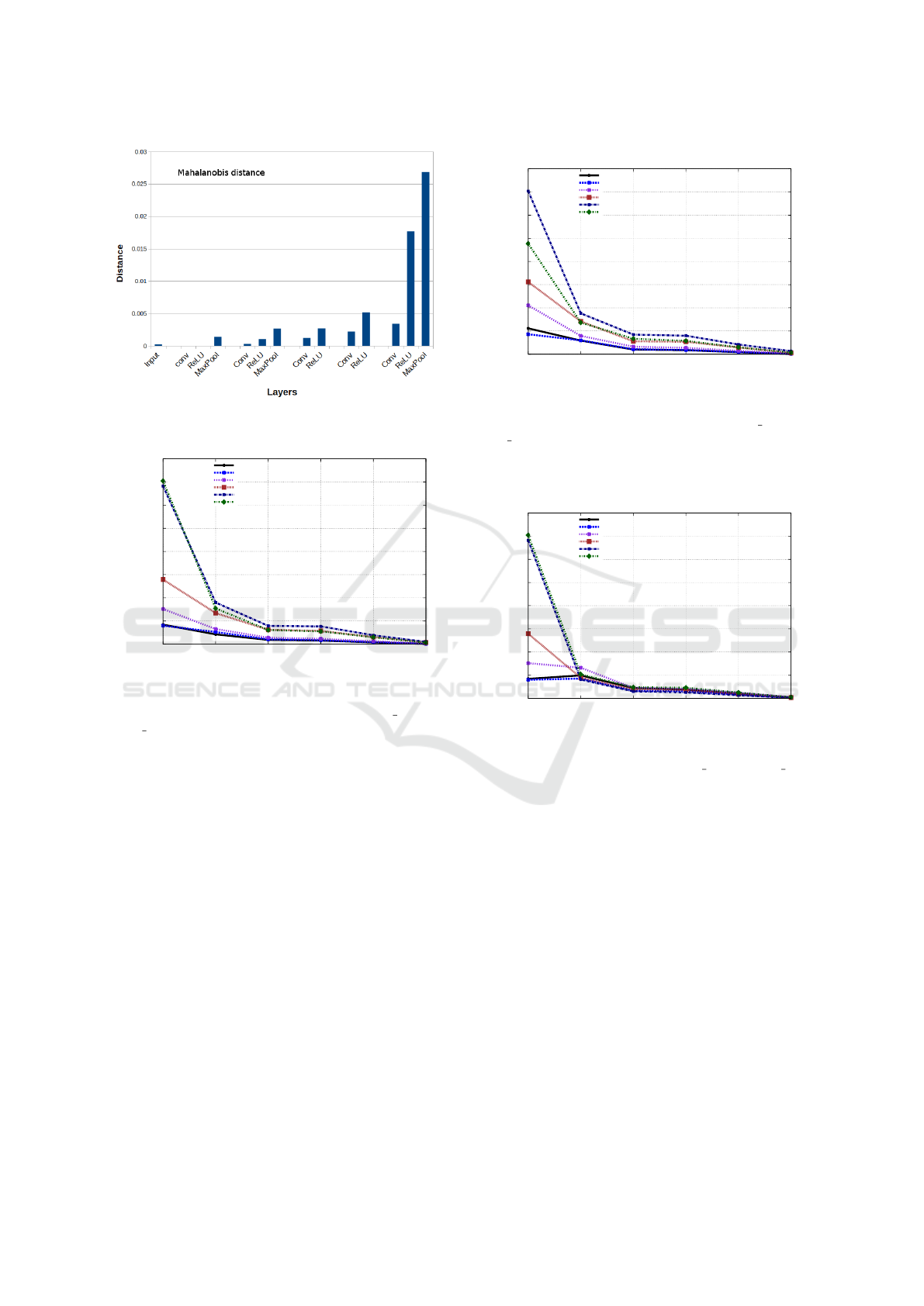
Figure 4: Mahalanobis distance between mean of classes.
0
10000
20000
30000
40000
50000
60000
70000
80000
0 1 2 3 4 5
Distance
Layers
Euclidean distance from mean
Near_Min
Medium_Min
Far_Min
Near_Max
Medium_Max
Far_Max
Figure 5: Euclidean distance of representative points from
mean (class 1). The first entry in x−axis shows the input
value followed by five layers of AlexNet. Near min and
Near max are minimum and maximum distance values, re-
spectively from the near region. Similarly for medium and
far regions the minimum and maximum values are shown.
spective means are getting reduced as points passes
through the subsequent layers. This reflects that the
points from same class are getting clustered together.
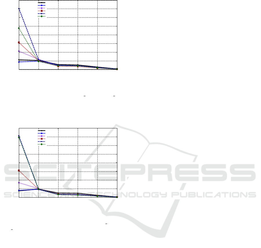
4.4 Euclidean Distance between
Representative Points within and
Across Classes
We also analyze how the distance between repre-
sentative points are changing after passing through
each subsequent layer. It is seen from Fig.7, Fig.8
and Fig.9 the distances among points within a class
decrease but distances among points between two
classes also reduce.
Even though distances between points from two
classes is also decreasing we can say that the network
is doing good classification as the other parameters
which we have seen such as the Mahalanobis distance
0
10000
20000
30000
40000
50000
60000
70000
80000
0 1 2 3 4 5
Distance
Layers
Euclidean distance from mean
Near_Min
Medium_Min
Far_Min
Near_Max
Medium_Max
Far_Max
Figure 6: Euclidean distance of representative points from
mean (class 2). The first entry in x−axis shows the input
value followed by five layers of AlexNet. Near min and
Near max are minimum and maximum distance values, re-
spectively from the near region. Similarly for medium and
far regions the minimum and maximum values are shown.
0
10000
20000
30000
40000
50000
60000
70000
80000
0 1 2 3 4 5
Distance
Layers
Euclidean Distance
Near_Min
Medium_Min
Far_Min
Near_Max
Medium_Max
Far_Max
Figure 7: Euclidean distance among representative points
(class 1). The first entry in x−axis shows the input value
followed by five layers of AlexNet. Near min and Near max
are minimum and maximum distance values, respectively
from the near region. Similarly for medium and far regions
the minimum and maximum values are shown.
between the means, singular values of the transfor-
mation matrix for the filters, increase of the angles
between points between two classes indicate that the
two classes are getting apart as they pass through the
layer of the network.
5 CONCLUSION
In this study, we consider the architecture of AlexNet
and its linear and nonlinear transformation operations.
We analyze the required criterion of transformation
matrix for appropriate classification and see that the
conditions are met fully for the last layer and par-
tially for the intermediate layers. We select six rep-
ICPRAM 2019 - 8th International Conference on Pattern Recognition Applications and Methods
864

0
10000
20000
30000
40000
50000
60000
70000
80000
0 1 2 3 4 5
Distance
Layers
Euclidean Distance
Near_Min
Medium_Min
Far_Min
Near_Max
Medium_Max
Far_Max
Figure 8: Euclidean distance among representative points
(class 2). The first entry in x−axis shows the input value
followed by five layers of AlexNet. Near min and Near max
are minimum and maximum distance values, respectively
from the near region. Similarly for medium and far regions
the minimum and maximum values are shown.
0
10000
20000
30000
40000
50000
60000
70000
80000
0 1 2 3 4 5
Distance
Layers
Euclidean Distance
Near_Min
Medium_Min
Far_Min
Near_Max
Medium_Max
Far_Max
Figure 9: Euclidean distance among representative points
(between classes). The first entry in x−axis shows the in-
put value followed by five layers of AlexNet. Near min and
Near max are minimum and maximum distance values, re-
spectively from the near region. Similarly for medium and
far regions the minimum and maximum values are shown.
resentative points from each class and observe the ef-
fect of nonlinear transformations on the input data by
measuring the change in angle and distance between
these points and we observed that same class data is
bunched together and different class data are well sep-
arated in-spite of the fact that all data points come
closer irrespective of class.
REFERENCES
Deng, J., Dong, W., Socher, R., jia Li, L., Li, K., and Fei-
fei, L. (2009). Imagenet: A large-scale hierarchical
image database. In In CVPR.
Dosovitskiy, A. and Brox, T. (2016). Inverting visual repre-
sentations with convolutional networks. In Proceed-
ings of the IEEE Conference on Computer Vision and
Pattern Recognition, pages 4829–4837.
Giryes, R., Sapiro, G., and Bronstein, A. M. (2016). Deep
neural networks with random gaussian weights: a uni-
versal classification strategy? IEEE Trans. Signal
Processing, 64(13):3444–3457.
Kim, H., Nam, H., Jung, W., and Lee, J. (2017). Perfor-
mance analysis of cnn frameworks for gpus. Perfor-
mance Analysis of Systems and Software (ISPASS).
Kobayashi, T. (2018). Analyzing filters toward efficient
convnet. In Proceedings of the IEEE Conference
on Computer Vision and Pattern Recognition, pages
5619–5628.
Krizhevsky, A., Sutskever, I., and Hinton, G. E. (2012). Im-
agenet classification with deep convolutional neural
networks. In Advances in neural information process-
ing systems, pages 1097–1105.
LeCun, Y., Boser, B., Denker, J. S., Henderson, D., Howard,
R. E., Hubbard, W., and Jackel, L. D. (1989). Back-
propagation applied to handwritten zip code recogni-
tion. Neural computation, 1(4):541–551.
Oyallon, E. (2017). Building a regular decision bound-
ary with deep networks. In 2017 IEEE Conference
on Computer Vision and Pattern Recognition (CVPR),
volume 00, pages 1886–1894.
Sokoli
´
c, J., Giryes, R., Sapiro, G., and Rodrigues, M. R.
(2017). Robust large margin deep neural net-
works. IEEE Transactions on Signal Processing,
65(16):4265–4280.
Sokoli
´
c, J., Giryes, R., Sapiro, G., and Rodrigues, M. R. D.
(2017). Generalization error of deep neural networks:
Role of classification margin and data structure. In
2017 International Conference on Sampling Theory
and Applications (SampTA), pages 147–151.
Xie, L., Zheng, L., Wang, J., Yuille, A. L., and Tian, Q.
(2016). Interactive: Inter-layer activeness propaga-
tion. In Proceedings of the IEEE Conference on Com-
puter Vision and Pattern Recognition, pages 270–279.
Young, T., Hazarika, D., Poria, S., and Cambria, E. (2018).
Recent trends in deep learning based natural language
processing. ieee Computational intelligenCe maga-
zine, 13(3):55–75.
Analyzing the Linear and Nonlinear Transformations of AlexNet to Gain Insight into Its Performance
865