Gradient Descent Analysis: On Visualizing the Training of Deep Neural
Networks
Martin Becker, Jens Lippel and Thomas Zielke
University of Applied Sciences D
¨
usseldorf, M
¨
unsterstr. 156, 40476, D
¨
usseldorf, Germany
Keywords:
Deep Neural Networks, Learning Process Visualization, Machine Learning, Numerical Optimization,
Gradient Descent Methods.
Abstract:
We present an approach to visualizing gradient descent methods and discuss its application in the context
of deep neural network (DNN) training. The result is a novel type of training error curve (a) that allows
for an exploration of each individual gradient descent iteration at line search level; (b) that reflects how a
DNN’s training error varies along each of the descent directions considered; (c) that is consistent with the
traditional training error versus training iteration view commonly used to monitor a DNN’s training progress.
We show how these three levels of detail can be easily realized as the three stages of Shneiderman’s Visual
Information Seeking Mantra. This suggests the design and development of a new interactive visualization
tool for the exploration of DNN learning processes. We present an example that showcases a conceivable
interactive workflow when working with such a tool. Moreover, we give a first impression of a possible DNN
hyperparameter analysis.
1 INTRODUCTION
Deep neural networks (DNNs) are machine learning
models that have demonstrated impressive results on
various real-world data processing tasks; yet their
widespread use is hampered due to the absence of a
generally applicable learning procedure. Usually, the
efficiency and robustness of deep learning processes
depend on a set of hyperparameters. Adjusting these
hyperparameters can be quite challenging, especially
for users who have only very little to no experience
with DNNs.
A standard strategy to assess learning processes
resulting from different hyperparameter settings is to
compare their training error curves. Although such a
comparison can help to gain a certain intuition about
individual hyperparameters and their interaction, it
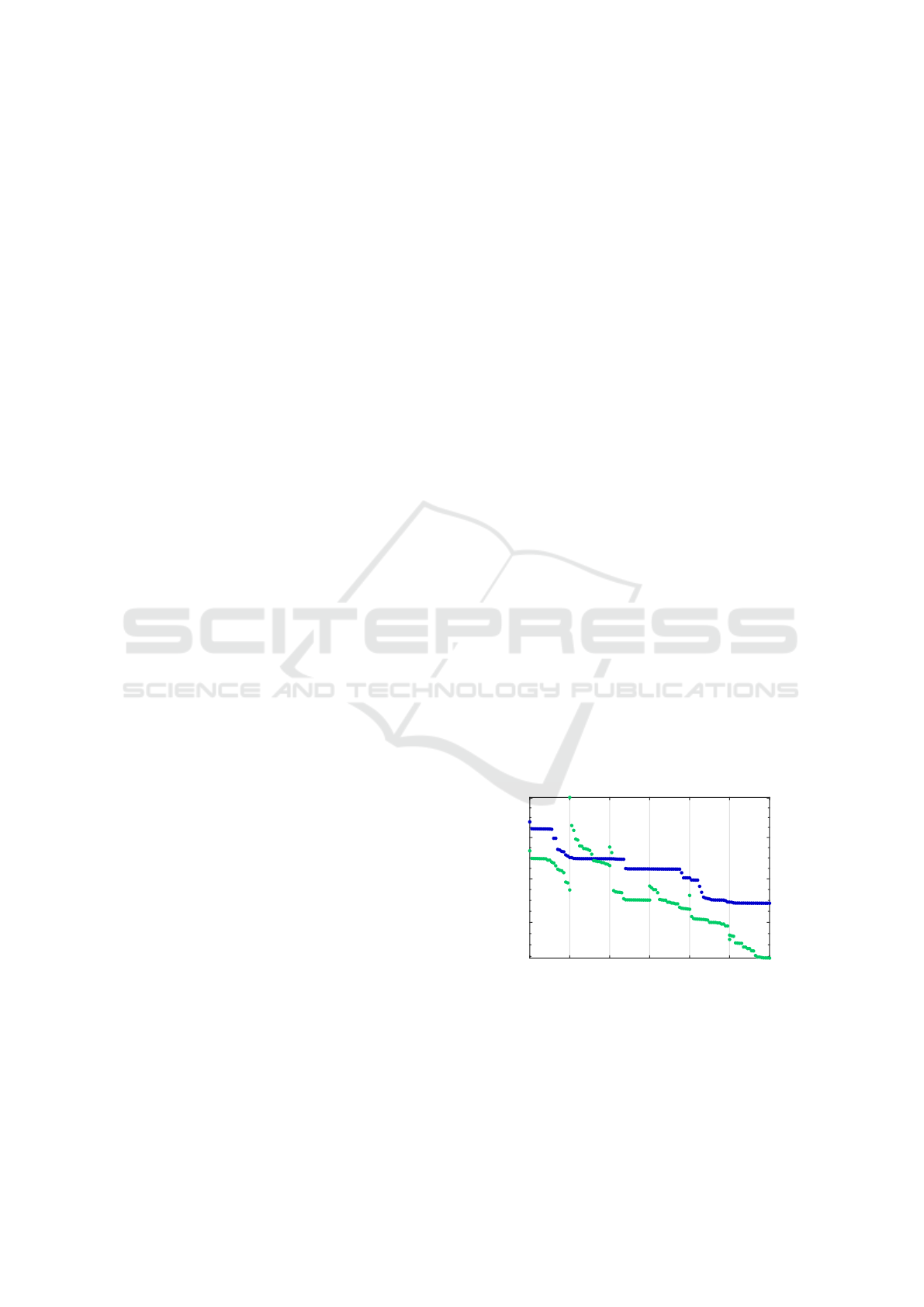
provides a fairly limited view on DNNs. E.g. Figure
1 shows two training error curves that we discuss in
Section 3. By comparing the two curves, we merely
learn how to differentiate between favorable training
error curves and less favorable ones but not how they
relate to the core mechanisms of deep learning.
In search of such a relation, we developed a novel
enhanced type of training error curve. It consists of
three levels of detail, which can be easily assigned
to the three stages of the Visual Information Seeking
Mantra (Shneiderman, 1996): In the overview stage,
the traditional training error curve is in the focus of
attention. In the zoom and filter stage, one can look
at the variation of the training error along each of
the descent directions considered during the gradient
descent-based DNN training. The details-on-demand
stage allows for an in-depth exploration of methods
0 20 40 60 80 100 120
0.38
0.4
0.42
0.44
Figure 1: Two exemplary training error curves. They show
a training error versus training iteration view. Displaying
them at the same time allows for a direct comparison. The
green curve has a smaller final error. At the same time, its
curve progression is more irregular as compared to the blue
curve, which appears to be decreasing monotonically. The
underlying core deep learning mechanisms remain unclear
because they are not directly accessible through a simple
comparison of the two training error curves.
338
Becker, M., Lippel, J. and Zielke, T.
Gradient Descent Analysis: On Visualizing the Training of Deep Neural Networks.
DOI: 10.5220/0007583403380345
In Proceedings of the 14th International Joint Conference on Computer Vision, Imaging and Computer Graphics Theory and Applications (VISIGRAPP 2019), pages 338-345
ISBN: 978-989-758-354-4
Copyright
c
2019 by SCITEPRESS – Science and Technology Publications, Lda. All rights reserved

for adaptive control of the step width along a given
descent direction.
The main intent of this paper is to introduce this
three-level / three-stage visualization approach in a
way that is comprehensible to both non-experts and
experts in the field of deep learning. To this end, we
begin by looking at an easy to understand non-DNN
example. It reflects all central elements of an actual
gradient descent-based DNN training but to a more
manageable extent. This also allows us to showcase
an interactive workflow that covers all three levels of
detail. The design and development of an interactive
tool for the visual exploration of the novel enhanced
training error curve is one of the goals of our future
work. We therefore also give a first impression of a
conceivable DNN hyperparameter analysis. We look
at the mini-batch size and show that varying it has a
very distinctive effect on a DNN’s enhanced training
error curve. This effect is not necessarily evident in
the overview stage but easy to spot in the zoom and
filter stage of our visualization approach. From this,
we conclude that our enhancement of the traditional
training error curve enables a more direct access to
DNN learning processes at hyperparameter level.
Over the last few years, visualization approaches
that help to better understand deep learning models
have been of great interest – a thorough overview of
the most recent approaches is presented in (Hohman
et al., 2018). However, it appears to us that gradient
descent methods have mainly been visualized to find
out what individual neurons can learn from data. By
contrast, our approach focuses on details relating to
the basic theoretical ideas behind a gradient descent
Table 1: A overview of gradient descent methods that we
intend to include in our interactive visualization tool. The
methods in the second table were specifically designed to
serve the needs of up-to-date deep learning models.
In this paper
Method Reference
Polak-Ribi
`
ere
(Polak and Ribi
`
ere, 1969)
CG method
∗
∗
) See (Polak, 2012) for an explanation in English.
Subject to future work
Method Reference
Rprop
∗∗
(Riedmiller, 1994)
AdaGrad (Duchi et al., 2011)
AdaDelta (Zeiler, 2012)
Adam and
(Kingma and Ba, 2014)
AdaMax
Nadam (Dozat, 2016)
AMSGrad (Reddi et al., 2018)
∗∗
) See (Igel and H
¨
usken, 2003) for different Rprop variants.
method. As a consequence, it can be applied to both
non-DNN and DNN scenarios. Table 1 lists some of
the gradient descent methods that we aim to include
in our interactive tool. In this paper, we consider the
Polak-Ribi
`
ere conjugate gradient (CG) method. The
methods in the second table are of special interest to
us because they were specifically designed to serve
the needs of up-to-date deep learning models. Their
study and inclusion in our visualization approach is
subject to future work.
2 VISUALIZATION APPROACH
As mentioned above, our visualization approach can
be applied to both non-DNN and DNN scenarios. In
general, it is applicable to virtually any problem that
can be modeled as follows:
Each solution to the problem can be represented
as a vector θ
θ
θ ∈ Θ where Θ := R
p
denotes the space
of possible solutions. One can define a continuously
differentiable error function J : Θ → R that enables
the assessment of each θ
θ
θ ∈ Θ; any optimal solution
θ
θ
θ
∗
∈ Θ satisfies
J(θ
θ
θ
∗
) ≤ J(θ
θ
θ) (∀θ
θ
θ ∈ Θ). (1)
We call any such θ
θ
θ
∗
a minimizer. In most cases,
the problem of finding minimizers cannot be solved
analytically. Here, gradient descent methods can be
applied in order to obtain good approximations.
Throughout this section, we consider an example
from a non-DNN context. The visualizations shown,
are based on results obtained through a CG descent
that we applied on J : R
2
→ [0|∞) defined by
J(θ
θ
θ) := 100(θ
2
− θ
2
1
)
2
+ (1 − θ
1
)
2
(2)
for θ
θ
θ ∈ Θ; its only minimizer (1, 1)
tr
is located in a
strongly curved valley following the parabola given
by θ
2
= θ
2
1
, which makes it difficult to approximate
(Rosenbrock, 1960). Because we are not looking at
an actual DNN training, we simply write traditional
and enhanced error curve.
2.1 Overview
For a given initial solution θ
θ
θ
0
∈ Θ, gradient descent
methods try to approximate minimizer by visiting a
finite sequence of solutions (θ
θ
θ
k
)
K
k=0
such that
J(θ
θ
θ
k+1
) < J(θ
θ
θ
k
) (∀k ∈ {0,... ,K − 1}). (3)
Because Rosenbrock’s function is a function of only
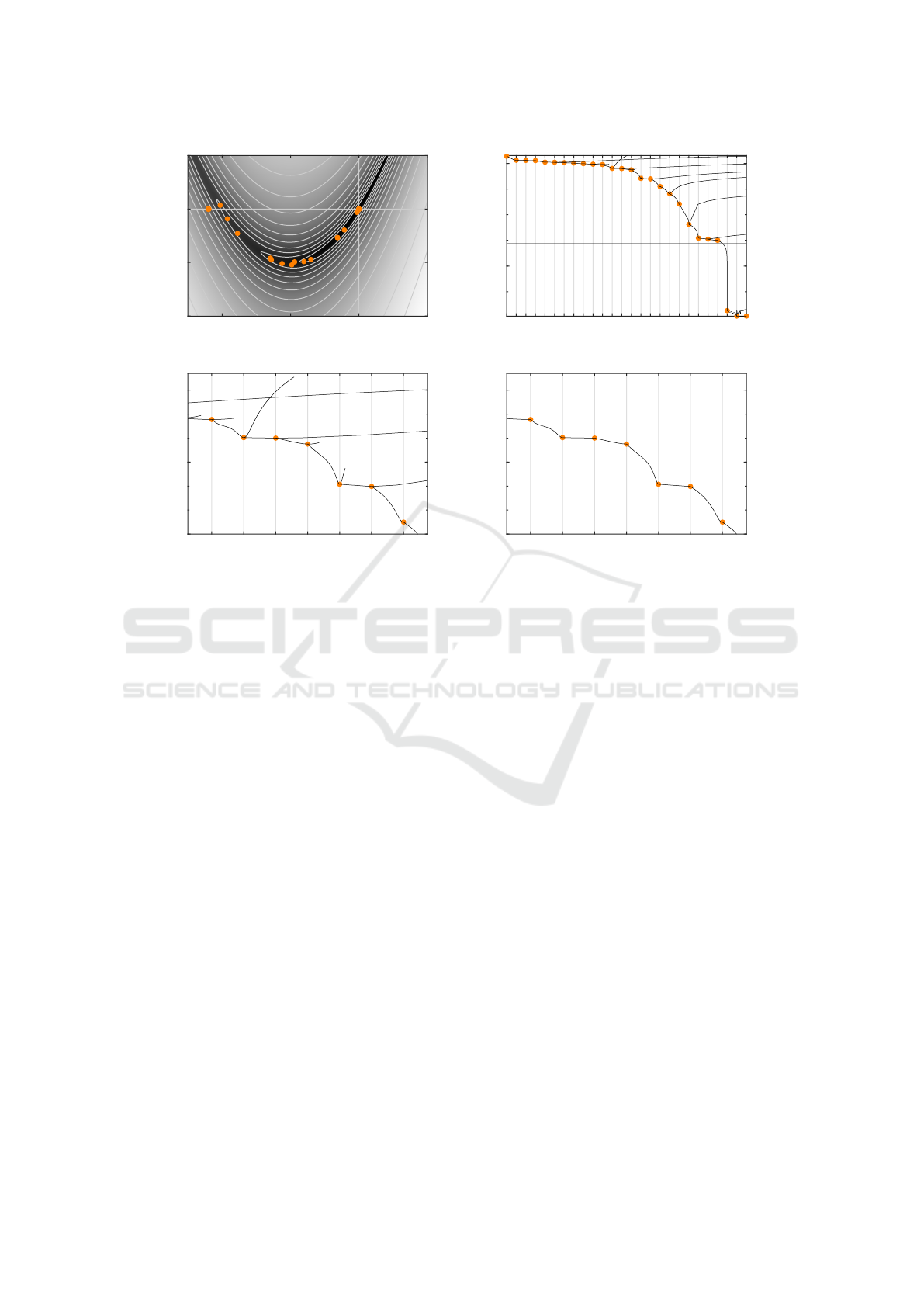
two variables, we can illustrate the visited solutions
as marks on a map. Figure 2(a) shows a heat map /
Gradient Descent Analysis: On Visualizing the Training of Deep Neural Networks
339
-1 0 1 2
-1
0
1
2
(a) Heat map / contour line plot.
0 5 10 15 20 25
10
-20
10
0
machine precision
(b) Overview.
10 11 12 13 14 15 16
10
-5
10
-2
10
1
(c) Zoom.
10 11 12 13 14 15 16
10
-5
10
-2
10
1
(d) Zoom and filter.
Figure 2: Visualizations of the results of the CG descent that we applied to Rosenbrock’s function (Rosenbrock, 1960). We
considered θ
θ
θ
0
:= (−1.2,1)
tr
as the initial solution. The views presented in (b), (c) and (d) give an impression of the overview
and zoom and filter stage of our visualization approach. The visualization tool that we are currently working on allows for an
interactive exploration of these views.
contour line plot of J. The marks are represented as
orange dots. We considered θ
θ
θ
0
:= (−1.2,1)
tr
as the
initial solution for the applied CG descent.
Figure 2(b) displays the corresponding overview
stage. The traditional error curve is in the focus of
attention of this view. It is simply the graph of the
mapping k 7→ J(θ
θ
θ
k
). Because this can be seen as an
another perspective on the information presented in
Figure 2(a), we use orange dots to depict the points
that form this graph. Assuming a machine precision
of about 10
−16
, we can safely state that ≈ 10
−15
(at
iteration 22) is the final approximation error.
The graphical elements that we added to obtain
the novel error curve are black curve segments. The
overview stage does not give us a clear enough view
on these segments, which is why we explain them in
the next section. However, there is one useful aspect
that is easy to comprehend without explanation: Note
that for errors lying significantly below the assumed
machine precision, the shape of the curve segments
reflect the resulting numerical noise. Because these
last two segments are the only ones to exhibit such a
behavior, it indicates either a successful descent or a
descent that ran into numerical difficulties. A future
study involving real-word data has to prove whether
the observed noise is distinctive enough to serve as
a reliable indicator of such cases. Clearly, studies of
this kind must include an investigation of individual
curve segments. The zoom and filter stage presented
in the next section is a step in that direction.
2.2 Zoom and Filter
Zooming in yields a clearer view on the black curve
segments. We explain what they represent using the
zoom view shown in Figure 2(c).
As a first step, we give a review on how gradient
descent methods get from solution to solution. The
key to this is the update rule
θ
θ
θ
k+1
:= θ
θ
θ
k
+ η
k
d
d
d
k
(4)
where d
d
d
k
∈ Θ must be a descent direction at θ
θ
θ
k
, i.e.
there has to exist a
¯
η
k
> 0 such that
J(θ
θ
θ
k
+ ηd
d
d
k
) < J(θ
θ
θ
k
) (∀η ∈ (0,
¯
η
k
]). (5)
Observe that constraining d
d
d
k
in this way guarantees
that inequality (3) is always satisfied for a range of
arbitrarily small step widths η > 0.
In the case of the CG descent, the step widths η
k
are determined through line searches that solve the
IVAPP 2019 - 10th International Conference on Information Visualization Theory and Applications
340
approximation problem
η
k
:≈ min {η > 0 | ϕ
0
k
(η) = 0 } (6)
where ϕ
k
: (0|∞) → R is defined by
ϕ
k
(η) := J(θ
θ
θ
k
+ ηd
d
d
k
) (η ∈ (0|∞)). (7)
The functions ϕ
k
reflect how J varies when we move
along d
d
d
k
starting at θ
θ
θ
k
. Each of them corresponds to
a curve segment in Figure 2(c). We look closer at the
curve segment that starts at (10,J(θ
θ
θ
10
)). It depicts a
horizontally translated and scaled version of ϕ
10
. We
know that η = η
10
must yield J(θ
θ
θ
11
). This follows
from the applied update rule (4). The approximation
rule (6), on the other hand, suggests that η
10
should be
chosen as the smallest stationary point of ϕ
10
, i.e. η
10
very likely indicates a local minimum – and less likely
a saddle point – of ϕ
10
. Indeed, the curve segment’s
minimum coincides with (11,J(θ
θ
θ
11
)). Thus, the part
of this curve segment that connects (10, J(θ
θ
θ
10
)) and
(11,J(θ
θ
θ
11
)) reflects the error variation when moving
from solution θ
θ
θ
10
to solution θ
θ
θ
11
. The rest (or loose
end) of the curve segment reflects how ϕ
10
varies in
the range from η
10
to η
max
10
where η
max
10
denotes the
maximum step width considered during the applied
line search. The applied line search is explained in
the next section.
Mathematically, the black curve segments show
the graphs of the functions c
k
: (k|ξ
max
k
] → R given
by
c
k
(ξ) := ϕ
k
((ξ − k)η
k
) (ξ ∈ (k|ξ
max
k
]) (8)
where ξ
max
k
:= k + η
max
k
/η
k
. Following the notation
established in the above example, η
max
k
denotes the
maximum step width considered during the applied
line search in iteration k.
Note that c
15
has no loose end, i.e. ξ
max
15
= 16. An
interesting filtering of the enhanced error curve is to
remove all loose ends, as shown in Figure 2(d). It has
become common practice to connect the orange dots
that form the traditional error curve by simply using
line segments. It is important to note that the shown
zoom and filter view presents a more truthful way of
connecting the orange dots.
2.3 Details-on-Demand
Now, that we understand what the novel black curve
segments represent and how they are constructed, we
can explore them individually. In the following two
sections, we look at the curve segments representing
ϕ
10
and ϕ
15
. Because we already discussed them in
the previous section, their analysis in this final stage
can be understood as the final step of the interactive
workflow that we intended to present.
We use these two concrete examples to illustrate
the applied line search. It consists of two phases. The
first phase is always entered, the second one is only
entered if necessary. In the case of a line search that
only involves phase one, the resulting curve segment
has no loose ends. Therefore, the two example curve
segments allow us to explain under which conditions
the second phase must be entered.
So far, we discussed the central idea of moving
from solution to solution in order to approximate an
optimal solution θ
θ
θ
∗
∈ Θ. Searching for a step width
can be imagined similarly. For each k ∈ {0, ... ,K},
the applied line search seeks to find η
k
by visiting a
finite sequence of step widths (η
j
k
)
J
j=0
where
η
0
k
:=
1
1 + kd
d
d
k
k
2
(9)
is set as the initial step width.
2.3.1 Phase One Only
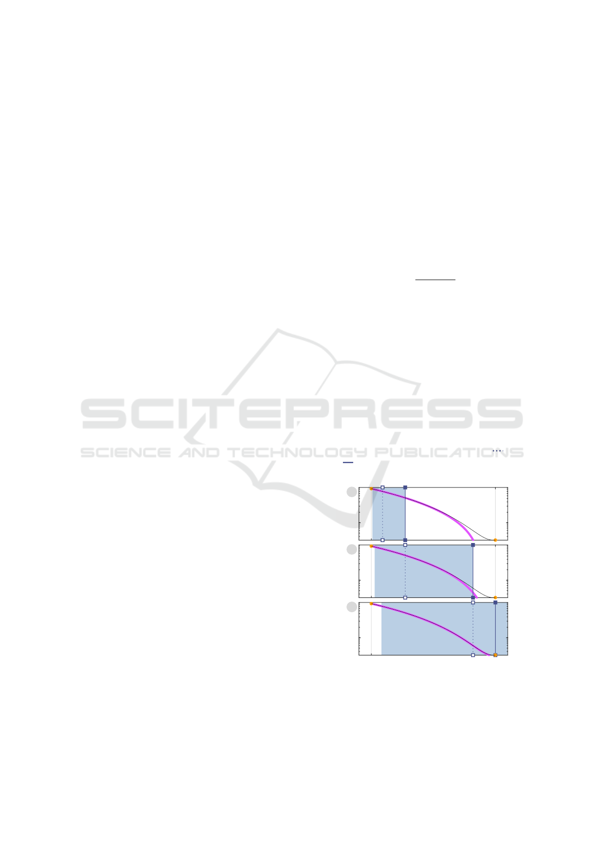
We begin by looking at the case k = 15 because we
know that the associated line search only involved
phase one. In Figure 3, the three iterations that were
needed to find η
15
are represented as three vertically
arranged plots. The annotated gray circles in the top
left corner of each plot indicate the index j. In the
following, we discuss them plot by plot. Parallel to
this, we explain the new graphical elements that are
provided by this details-on-demand view.
The vertical lines mark the current (
) and
next (
) step width; in the upper plot we see η
0
15
15 16
10
-4
1
15 16
10
-4
2
15 16
10
-4
3
Figure 3: Details-on-demand view of the curve segment
representing ϕ
15
. The three plots show the three iterations
needed to determine η
15
. This is an example of a line search
that only involves phase one. Such curve segments do not
have a loose end. See Figure 4 for an example of a curve
segment with a loose end.
Gradient Descent Analysis: On Visualizing the Training of Deep Neural Networks
341
and η
1
15
, respectively. In general, the magenta curve
represents the cubic polynomial π that is obtained
through a Hermite interpolation with respect to
π(0) = ϕ
k
(0) π(η
j
k
) = ϕ
k
(η
j
k
) (10)
π
0
(0) = ϕ
0
k
(0) π
0
(η
j
k
) = ϕ
0
k
(η
j
k
) (11)
where η
j
k
denotes the current step width. Clearly, the
current control points 0 and η
0
15
provide very limited
view on ϕ
15
. However, π already well-approximates
ϕ
15
. The idea behind π is to find its minimizer and
limit it through the interval that is indicated by the
light blue area. The result is then set as the next step
width. As can be seen, η
∗
exceeds the upper bound
of the interval because the upper bound is marked by
, i.e. it was set as the next step width η
1
15
.
Because the three plots are vertically aligned and
share the same axis limits, we directly see that η
1
15
severs as the current (
) step width in the middle
plot. It is also easy to see that π is now an even better
approximation of ϕ
15
; yet still its minimizer η
∗
is too
large. Again, the upper bound of the interval that is
indicated by the light blue area is set as the next step
width η
2
15
. The interval is expanded as compared to
the upper plot. In general, the interval is defined by
[αη
j
k
|βη
j
k
] with 0 < α < 1 < β. In our case, we have
α := 0.1 and β := 3.0. This explains the expansion
of the interval. The interval length grows with the
current step width. At the beginning, we consider a
small initial step width and we also ensure that we do
not move too fast.
Finally, π approximates ϕ
15
to an extent where
their minimums coincide. Furthermore, the light blue
area is contains this minimum. The minimizer η
∗
is
set as the next step width η
3
15
and also as the step
width η
15
since ϕ
0
15
(η
3
15
) ≈ 0.
2.3.2 Phase One and Phase Two
Curve segments with loose ends result from moving
too far along the respective function ϕ
k
, i.e. we move
past the desired minimizer η
k
of ϕ
k
and have to find
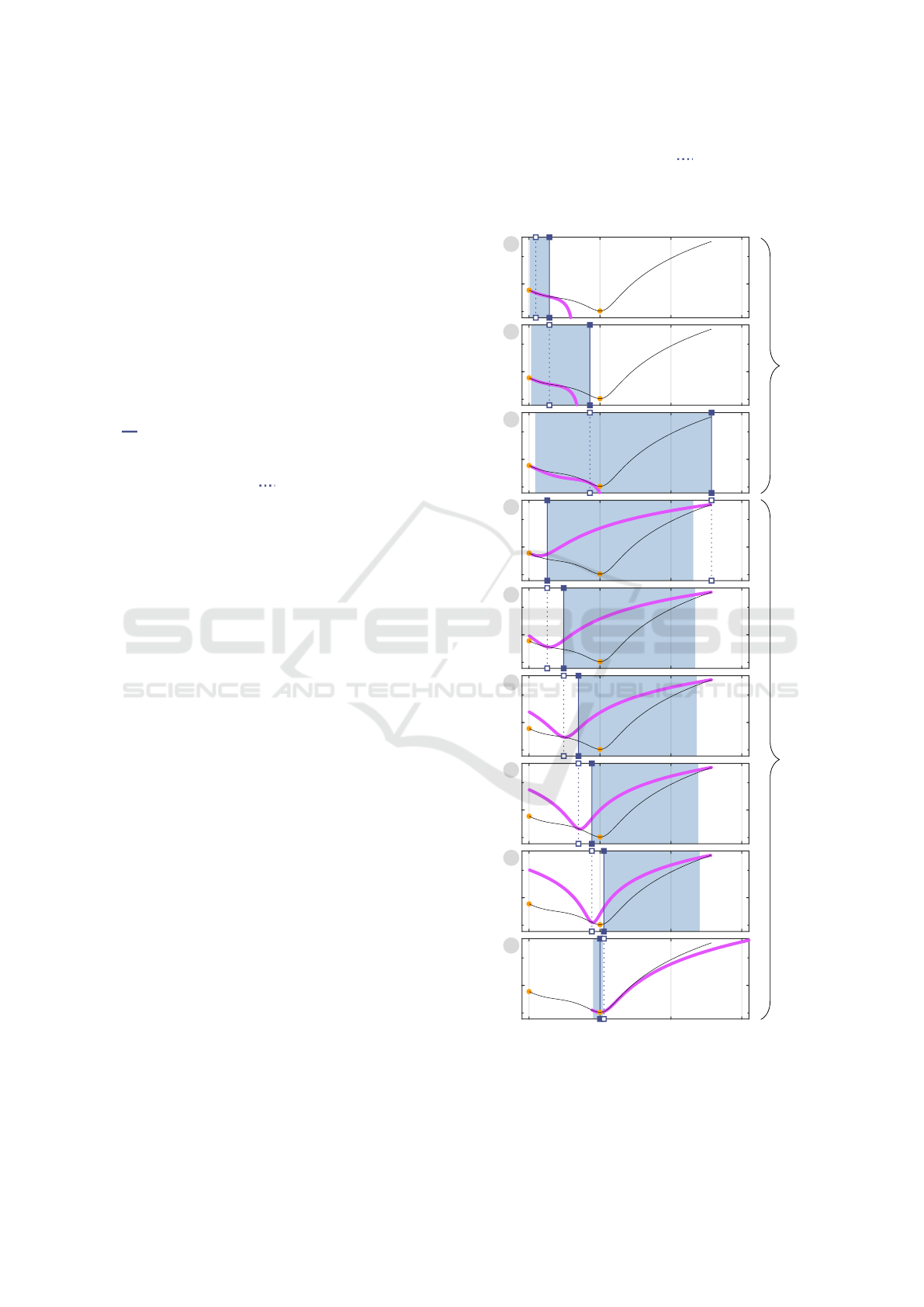
our way back. We look at the case k = 10. Figure 4
shows all iterations that were carried out.
The first three plots show the iterations of phase
one. During phase one, the upper bound of the light
blue area is set as the next step width three times in
a row. In contrast to the previous example, this is
not because the respective minimizers η
∗
of π are too
large. The minimizers simply do not exist in the first
three cases. At the end of iteration three, we are to the
right of the minimizer η
10
of ϕ
10
.
Now, phase two uses that phase one is exited at
any step width η
j
k
with ϕ
0
k
(η
j
k
) > 0. Clearly, the slope
at the current step width η
3
10
(
) in iteration four
is positive. Moreover, since ϕ
10
reflects how J varies
along a descent direction, it is also always true that
10 11 12 13
10
0
1
10 11 12 13
10
0
2
10 11 12 13
10
0
3
10 11 12 13
10
0
4
10 11 12 13
10
0
5
10 11 12 13
10
0
6
10 11 12 13
10
0
7
10 11 12 13
10
0
8
10 11 12 13
10
0
9
Phase one
Phase two
Figure 4: Details-on-demand view of the curve segment
representing ϕ
10
. The nine plots show the three iterations
needed to determine η
10
. Phase two is entered because
phase one visits a step width that lies to the right of the
minimizer η
10
of ϕ
10
.
IVAPP 2019 - 10th International Conference on Information Visualization Theory and Applications
342
ϕ
0
10
(η) < 0 for η → 0. So, η
10
must lie in (a|b) with
a = 0 and b = η
3
10
. The central idea behind phase two
is to gradually shrink the interval (a|b) while ensuring
that ϕ
0
10
(a) < 0 and ϕ
0
10
(b) > 0. Table 2 summarizes
the interval updates. Moreover, it reveals that phase
two involves two types of Hermite interpolation:
In the iterations four to eight, the magenta curve
represents a quadratic polynomial π. As in phase one,
a minimizer η
∗
of π is determined and limited through
the interval that is indicated by the light blue area. In
the case of the iterations four to eight, the minimizer
η
∗
is always too small. Thus, the lower bound of the
corresponding interval is set as the next step width.
Here, the lower and the upper bound are given by a +
0.1(b − a) and b − 0.1(b − a), respectively.
Only in the final iteration, the magenta curve is
based on a cubic Hermite interpolation. The mini-
mums of the curve segment and the magenta curve
coincides and therefore the minimizer η
∗
is set as the
next step width η
9
10
and, moreover, η
9
10
is set as the
step width η
10
since ϕ
0
10
(η
9
10
) ≈ 0.
Table 2: An overview of the interval updates and the inter-
polation types applied in phase two.
Phase two
j a b Interpolation
4 0 η
3
10
ϕ
k
(η
j
k
) > ϕ
k
(0) ⇒ quadratic
w.r.t. ~
π(a) = ϕ
k
(a)
π
0
(a) = ϕ
0
k
(a)
π(b) = ϕ
k
(b)
5 η
4
10
η
3
10
6 η
5
10
η
3
10
7 η
6
10
η
3
10
8 η
7
10
η
3
10
ϕ
k
(η
j
k
) ≤ ϕ
k
(0) ⇒ cubic
w.r.t. ~ and π
0
(b) = ϕ
0
k
(b)
9 η
7
10
η
8
10
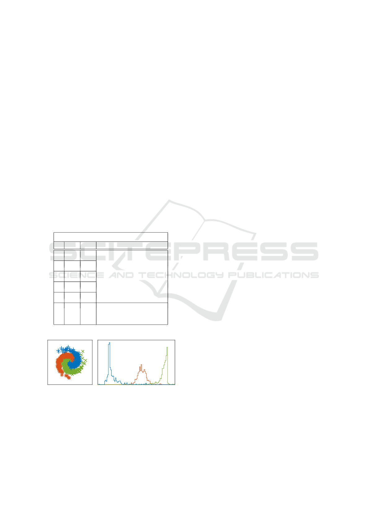
(a) Galaxy. (b) 1D visualization.
Figure 5: A scatter plot of the artificial galaxy data set and
a histogram of the 1D representation obtained through the
learned DNN mapping. Taken from (Becker et al., 2017).
3 A DNN EXAMPLE
An important application of DNNs that is especially
useful in the visualization context is the learning of
dimensionality reducing mappings. Such mappings
can yield 1D, 2D or 3D representations of original
high-dimensional data that allow for straightforward
visualizations such as histograms and scatter plots.
In (Becker et al., 2017), we introduced a robust
DNN approach to dimensionality reduction. To test
our implementation, we conducted a toy experiment
involving an artificially generated galaxy data set. In
Figure 5, we see one of the results of the paper. The
2D galaxy depicted in Figure 5(a) consists of three
classes each containing 480 samples. The suggested
DNN was used to learn a non-linear mapping to 1D.
The obtained 1D representation of the 2D galaxy is
shown Figure 5(b). In the displayed histogram, the
three classes are visually separable even without the
applied color scheme.
Subsequently, we use this DNN and this data set
to give a first impression of enhanced training error
curves of actual DNN learning processes. We show
two curves obtained through trainings with different
mini-batch sizes.
3.1 Batch and Mini-batch Training
Essentially, a DNN is a parametric machine learning
model covering an infinite number of mappings. Its
parameters are often formalized as a vector θ
θ
θ ∈ Θ
where Θ := R
p
is called the parameter space of the
DNN. The number p of parameters is implicitly set
by specifying the internal structure of a DNN. In the
context of this paper, a deeper understanding of this
internal structure is not required. See (Becker et al.,
2017) for a description and also for the definition of
the used error function J.
In a (real-world) deep learning scenario, J(θ
θ
θ
k
) is
used to assess the data processing
x
x
x
n
7→ z
z
z
n
:= f
f
f
θ
θ
θ
k
(x
x
x
n
) ∈ Z := R
d
Z
(12)
where {x
x
x
1
,.. ., x
x
x
N
} ⊂ X := R
d
X
is a set of training
samples and f
f
f
θ
θ
θ
k
: X → Z is the mapping associated
with the kth solution θ
θ
θ
k
∈ Θ visited during the DNN
training.
DNN training is commonly not performed using
all N training samples at once – this training strategy
is referred to as batch training. Instead, the training
samples are randomly split into B ≤ N subsets. Then
a gradient descent is performed based on one subset
at a time. Once all subsets have been presented for a
gradient descent, the set of training samples is again
randomly split for another B gradient descents. This
Gradient Descent Analysis: On Visualizing the Training of Deep Neural Networks
343
0 10 20 30 40 50 60 70 80 90 100 110 120
0.38
0.4
0.42
0.44
0.46
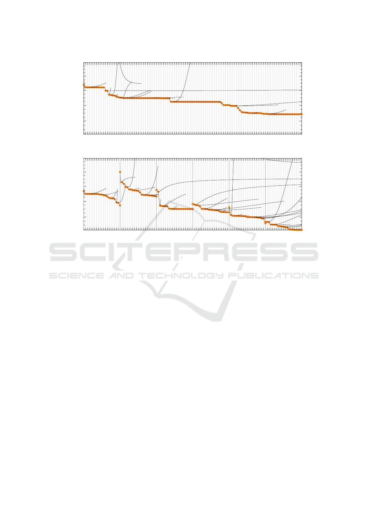
(a) Enhanced batch training error curve.
0 10 20 30 40 50 60 70 80 90 100 110 120
0.38
0.4
0.42
0.44
0.46
(b) Enhanced mini-batch training error curve.
Figure 6: Enhanced training error curves showing a zoom view on the first 120 gradient descent iterations of the batch training
and the mini-batch training, respectively. In the case of the mini-batch training, these 120 iterations result from the following
experimental setup: B = 3 mini-batches; 20 iterations per CG descent per mini-batch; 2 training epochs.
is repeated for several training epochs. For B strictly
smaller than N (ideally, N mod B = 0), each subset
is called a mini-batch, and accordingly, the training
strategy is called mini-batch training. Clearly, for B
equals 1, we obtain a batch training. The case B = N
leads to an online training, a training strategy that is
rarely used to date.
3.2 Experiments and Results
We conducted two new experiments: In the first, we
applied the batch training strategy. In the second, we
used the mini-batch training strategy with B = 3, i.e.
the individual gradient descents were performed on
the basis of mini-batches of the size 480. In order to
enable a fair comparison of the two experiments, we
ensured that each mini-batch contained 160 samples
of each of the three classes. Put differently, we made
sure that the class proportions were always the same
in both experiments.
Figures 6(a) and 6(b) show the zoom view of the
first 120 gradient descent iterations of the respective
enhanced training error curves – they correspond to
the blue and the green traditional curve displayed in
Figure 1. The enhanced batch training error curve is
displayed in Figure 6(a) and it reveals no substantial
differences from the enhanced error curve shown in
Figure 2(b). In both cases, the black curve segments
connect the points of the respective traditional curve
and they may or may not have loose ends. However,
it is striking that there exist several long runs of CG
descents that appear to cause no significant decrease
in error. This is due to the higher complexity of the
given deep learning problem.
The enhanced training error curve obtained from
the mini-batch training is depicted in Figure 6(b). It
strongly differs from both curves discussed so far. In
order to be able to interpret the main difference, we
need to further elaborate on our mini-batch training
realization: We chose to perform a constant number
of 20 iterations per CG descent per mini-batch. The
120 iterations therefore display two entire epochs of
mini-batch training or, respectively, six consecutive
CG descents. The slightly thicker vertical grid lines
mark the beginnings of these CG descents.
Now, a closer look along these thicker grid lines
reveals that the black curve segments already reflect
these beginnings of CG descents. There are distinct
IVAPP 2019 - 10th International Conference on Information Visualization Theory and Applications
344

discontinuities at the iterations 20, 40, 60, etc. This
can be explained by the fact that the error function
changes at these points. The error function of a DNN
ultimately depends on the presented sets of training
samples. While this is not a new insight, the views
that are provided by the enhanced training error curve
can help to study these effects in greater detail. E.g.
we can now look at how varying the mini-batch size
influences the shape of the functions ϕ
k
as regards
their change in steepness, smoothness, etc. We can
look at the same experiment but at the level of line
searches. Interesting new features are the number of
loose ends, the number line search iterations needed
on average etc. Another experiment is to vary K, the
number of iterations per CG descent per mini-batch,
or even some ratio of K and the mini-batch size. In
any scenario, our approach does not confront us with
views that we are unfamiliar with. Instead, we get an
extension of widespread monitoring tool and we can
access its novel features as needed.
4 CONCLUSION
In this paper, we presented a novel enhanced type of
the training error curve that consists of three levels
of detail. We showed how these levels of detail can
be organized as proposed by the Visual Information
Seeking Mantra (Shneiderman, 1996): The overview
stage covers the details of a traditional training error
versus training iteration view. At the same time, it is
marked by new graphical elements that can be easily
accessed through zooming and filtering. These new
elements reflect how the training error varies as we
move from solution to solution in a gradient descent
iteration. The details-on-demand view allows for an
exploration of the methods that determine how far to
move along a given descent direction.
We were able to give an example that covered all
levels of detail accessible through the novel training
error curve. Guided by Sheiderman’s Mantra, it was
possible to introduce our visualization approach in a
way that can be seen as an interactive workflow. The
design and development of an interactive tool for the
visual exploration of the novel training error curve is
one of our future goals. To this end, we identified a
list of other gradient descent methods that we aim to
include in our tool (see Table 1).
As a final step, we gave a first impression of a hy-
perparameter analysis that can be realized with our
visualization approach. In the course of this, we
hinted at further possibilities to gain new insights as
regards the mini-batch training of DNNs. While the
concrete experimental setup did not reveal entirely
new insights about mini-batch training approaches,
we pointed out that our way of visualizing gradient
descent-related quantities is especially useful since
users can access lower level details as needed and by
using a monitoring tool that feels familiar.
REFERENCES
Becker, M., Lippel, J., and Stuhlsatz, A. (2017). Regu-
larized nonlinear discriminant analysis - an approach
to robust dimensionality reduction for data visualiza-
tion. In Proceedings of the 12th International Joint
Conference on Computer Vision, Imaging and Com-
puter Graphics Theory and Applications - Volume
3: IVAPP, (VISIGRAPP 2017), pages 116–127. IN-
STICC, SciTePress.
Dozat, T. (2016). Incorporating nesterov momentum into
adam. ICLR Workshop Submission.
Duchi, J., Hazan, E., and Singer, Y. (2011). Adaptive sub-
gradient methods for online learning and stochastic
optimization. J. Mach. Learn. Res., 12:2121–2159.
Hohman, F., Kahng, M., Pienta, R., and Chau, D. H. (2018).
Visual analytics in deep learning: An interrogative
survey for the next frontiers. IEEE transactions on
visualization and computer graphics.
Igel, C. and H
¨
usken, M. (2003). Empirical evaluation of
the improved rprop learning algorithms. Neurocom-
puting, 50:105–123.
Kingma, D. P. and Ba, J. (2014). Adam: A method for
stochastic optimization. CoRR, abs/1412.6980.
Polak, E. (2012). Optimization: Algorithms and Consis-
tent Approximations. Applied Mathematical Sciences.
Springer New York.
Polak, E. and Ribi
`
ere, G. (1969). Note sur la conver-
gence de m
´
ethodes de directions conjugu
´
ees. ESAIM:
Mathematical Modelling and Numerical Analysis -
Mod
´
elisation Math
´
ematique et Analyse Num
´
erique,
3(R1):35–43.
Reddi, S. J., Kale, S., and Kumar, S. (2018). On the conver-
gence of adam and beyond. In International Confer-
ence on Learning Representations.
Riedmiller, M. (1994). Advanced supervised learning
in multi-layer perceptrons from backpropagation to
adaptive learning algorithms. Computer Standards &
Interfaces, 16(3):265 – 278.
Rosenbrock, H. H. (1960). An automatic method for finding
the greatest or least value of a function. The Computer
Journal, 3(3):175–184.
Shneiderman, B. (1996). The eyes have it: A task by data
type taxonomy for information visualizations. In Pro-
ceedings of the 1996 IEEE Symposium on Visual Lan-
guages, VL ’96, pages 336–, Washington, DC, USA.
IEEE Computer Society.
Zeiler, M. D. (2012). ADADELTA: an adaptive learning
rate method. CoRR, abs/1212.5701.
Gradient Descent Analysis: On Visualizing the Training of Deep Neural Networks
345
