Speeding Up Classifier Chains in Multi-label Classification
Jose M. Moyano
1
, Eva L. Gibaja
1
, Sebasti
´
an Ventura
1
and Alberto Cano
2
1
Dpt. of Computer Science and Numerical Analysis, University of C
´
ordoba, Spain
2
Dpt. of Computer Science, Virginia Commonwealth University, U.S.A.
Keywords:
Multi Label Classification, Distributed Computing.
Abstract:
Multi-label classification has attracted increasing attention of the scientific community in recent years, given
its ability to solve problems where each of the examples simultaneously belongs to multiple labels. From all
the techniques developed to solve multi-label classification problems, Classifier Chains has been demonstrated
to be one of the best performing techniques. However, one of its main drawbacks is its inherently sequential
definition. Although many research works aimed to reduce the runtime of multi-label classification algorithms,
to the best of our knowledge, there are no proposals to specifically reduce the runtime of Classifier Chains.
Therefore, in this paper we propose a method called Parallel Classifier Chains which enables the parallelization
of Classifier Chain. In this way, Parallel Classifier Chains builds k binary classifiers in parallel, where each
of them includes as extra input features the predictions of those labels that have been previously built. We
performed an experimental evaluation over 20 datasets using 5 metrics to analyze both the runtime and the
predictive performance of our proposal. The results of the experiments affirmed that our proposal was able
to significantly reduce the runtime of Classifier Chains while the predictive performance was not statistically
significantly harmed.
1 INTRODUCTION
One of the best known and widely studied tasks in
data mining is classification. The aim of this task is
to learn a model by a set of examples, each labeled
with one and only one class, which would be able
to predict the class for unseen examples. However,
in many real-world problems, the examples could not
only belong to one but to many classes (a.k.a. labels)
simultaneously. For example, in medicine, one pa-
tient could be diagnosed with several diseases at the
same time. This fact gave rise to a new paradigm
called Multi-Label Classification (MLC), which al-
lowed each example to be labeled with more than
one class label at the same time (Gibaja and Ven-
tura, 2014). MLC has been successfully applied to
many real-world problems such as social networks
mining (Tang and Liu, 2009), multimedia annota-
tion (Nasierding and Kouzani, 2010) and bioinformat-
ics (Brandt et al., 2014), among others.
The most basic method to tackle the MLC prob-
lem is Binary Relevance (BR) (Tsoumakas et al.,
2010), which builds an independent classifier for each
of the labels. However, the labels of a problem are
often related to each other and have statistical depen-
dencies among them. Thus, the fact of not consider-
ing these relationships could be a great obstacle in the
predictive performance of the model. In order to over-
come this main drawback of BR, some other methods
have been proposed in the literature, such as Classifier
Chains (CC) (Read et al., 2011). CC is based on the
idea of BR, but the classifiers are chained in such a
way that each classifier includes the predicted labels
from previous classifiers as extra input features. In
this way, CC is able to model the relationships among
labels but it still has two main drawbacks: 1) the order
of the chain could have a direct effect on the predic-
tive performance of the MLC model, and 2) as each
classifier needs the outputs of previous classifiers, the
different binary models could not be built in parallel.
In order to tackle the first problem, several approaches
have been proposed, particularly ensemble of random
chains (Read et al., 2011; Dembczynski et al., 2010;
Goncalves et al., 2015).
Furthermore, with the emergence of large-scale
multi-label datasets, and the so-called extreme multi-
label classification (Prabhu and Varma, 2014), the re-
duction of the runtime of MLC methods becomes nec-
essary. A large number of research works have pro-
posed different methodologies in order to improve the
runtime of MLC algorithms, from methods that use
distributed systems to speed up some state-of-the-art
Moyano, J., Gibaja, E., Ventura, S. and Cano, A.
Speeding Up Classifier Chains in Multi-label Classification.
DOI: 10.5220/0007614200290037
In Proceedings of the 4th International Conference on Internet of Things, Big Data and Security (IoTBDS 2019), pages 29-37
ISBN: 978-989-758-369-8
Copyright
c
 2019 by SCITEPRESS – Science and Technology Publications, Lda. All rights reserved
29

algorithms (Skryjomski et al., 2018; Gonzalez-Lopez
et al., 2017; Gonzalez-Lopez et al., 2018; Babbar
and Sch
¨
olkopf, 2017) to methods that reduce the la-
bel space aiming to obtain a lower runtime in the re-
duced dataset (Hsu et al., 2009; Charte et al., 2014).
However, to the best of our knowledge, no approaches
have been proposed to date in order to be able to par-
allelize or speed up CC, which has been demonstrated
to be one of the best performing MLC methods (Moy-
ano et al., 2018).
Therefore, the objective of this paper is to pro-
pose a modified version of the CC method in order
to make it parallelizable. Moreover, we also aim to
prove that this new method (hereafter called Paral-
lel Classifier Chains, PCC) significantly reduces the
time to build a CC classifier while not harming its
predictive performance. In PCC, k binary classifiers
are built in parallel, each introducing as extra input
features the predictions of all previous classifiers that
have already finished. In the beginning, k classifiers
that do not consider any label prediction as input fea-
ture are built, instead of only one as in CC. As a result,
each binary classifier will introduce less label infor-
mation as input features, so the dependencies among
labels might be modeled slightly worse. However, in
high-dimensional label spaces, this difference is neg-
ligible, and also it will depend on how many classi-
fiers are built in parallel.
The rest of the paper is organized as follows: Sec-
tion 2 presents related work. Section 3 introduces
the new proposed methodology to speed up the CC
method. Section 4 includes the experimental study as
well as the discussion of the results. Finally, Section 5
presents the conclusions of the paper.
2 RELATED WORK
Let be L = {λ
1
,λ
2
,··· , λ
q
}, with q > 1 the set of q
binary labels and X the set of m instances each com-
posed by d input features. Let be D a multi-label
dataset composed by m pairs (x
x
x,y
y
y), being x
x
x
i
∈ X each
of the m examples and y
y
y
i
⊆ L the set of relevant labels
associated to x
x
x
i
. The MLC task is defined as learning
a model from D that maps from an unseen example
x
x
x
i
to a set of predicted relevant labels
ˆ
y
y
y
i
(Gibaja and
Ventura, 2014).
Several methods have been proposed in the liter-
ature to tackle the MLC task. The simplest method
in MLC is Binary Relevance (BR) (Tsoumakas et al.,
2010). BR builds q independent binary classifiers,
one for each of the labels of the problem. BR is
a simple and intuitive method, nevertheless, it does
not really take advantage of the multi-label scenario,
since it does not consider the relationships among la-
bels, which harms the predictive performance in prob-
lems were labels are highly related among each other.
On the other hand, Label Powerset (LP) (Tsoumakas
and Katakis, 2007) transforms the multi-label prob-
lem into a multi-class one, where each unique com-
bination of labels becomes a new class. Since LP
already considers the relationship among labels, its
main drawback is that the complexity of the new out-
put space grows exponentially with the number of
labels, so it could make the problem unmanageable
in scenarios where the number of labels is relatively
large.
Many other methods have been proposed to over-
come the different issues of both BR and LP. Classi-
fier Chains (CC) (Read et al., 2011) is based on BR
but it creates a chain of binary classifiers in such way
that each classifier in the chain also includes as in-
put features the predictions of previous labels in the
chain. In this way, CC considers the relationships
among labels in a more relaxed way than LP but also
with a lower computational complexity in cases with
very large label spaces. However, CC also has many
drawbacks, as the order of the chain will have a di-
rect effect on its predictive performance. Further-
more, binary classifiers of CC could not be built in
parallel, unlike BR, whose classifiers could be paral-
lelized since they are totally independent. In order to
address the chain problem, some methods have been
proposed in order to obtain an optimal chain (Dem-
bczynski et al., 2010; Goncalves et al., 2015; Moyano
et al., 2017; Melki et al., 2017). Moreover, Read et
al. (Read et al., 2011) propose to use an Ensemble of
Classifier Chains (ECC). ECC constructs an ensem-
ble of n CCs, each with a different subset of the train-
ing data and also with a different label chain, which
could reduce the probability of selecting a bad chain
that would lead to a poor performance.
Pruned Sets (PS) (Read, 2008) was proposed
based on LP. In order to reduce the high complexity
of LP, PS prunes the combinations of labels that ap-
pear so infrequently but reintroducing instances with
more frequent subsets of the labels. Furthermore, they
propose to use an Ensemble of Pruned Sets (EPS),
where each of the n PSs is built with a different sub-
set of the training instances. Hierarchy Of Multi-label
classifiERs (HOMER) (Tsoumakas et al., 2008) gen-
erates a tree of multi-label classifiers, where the root
contains all labels and each leaf represents one label.
At each node, the labels are split with a clustering
algorithm, grouping similar labels into a meta-label.
Finally, RAndom k-labELsets (RAkEL) (Tsoumakas
et al., 2011a) builds an ensemble of LP classifiers,
where each of the members of the ensemble is built
IoTBDS 2019 - 4th International Conference on Internet of Things, Big Data and Security
30

over a random projection of the output space, so they
are able to model the dependencies among labels but
with a much lower computational complexity than LP.
A more extensive description of methods in MLC
can be found in (Gibaja and Ventura, 2014). How-
ever, in spite of the large number of methods to
tackle the MLC problem, both CC and ECC have
been demonstrated to be one of the best perform-
ing methods (Moyano et al., 2018). Therefore, given
the great predictive performance of CC method (and
those based on it) and the fact that CC is not paral-
lelizable, we aimed to propose a methodology or a
redefinition of CC in order to make it parallelizable
and speed up its runtime.
3 PARALLEL CLASSIFIER
CHAINS
The original definition of CC made it inherently
sequential and non-parallelizable since each binary
classifier needs the predictions of previous classifiers
in the chain. However, we propose to redefine or
soften the original definition of CC in order to be able
to build the binary classifiers in parallel.
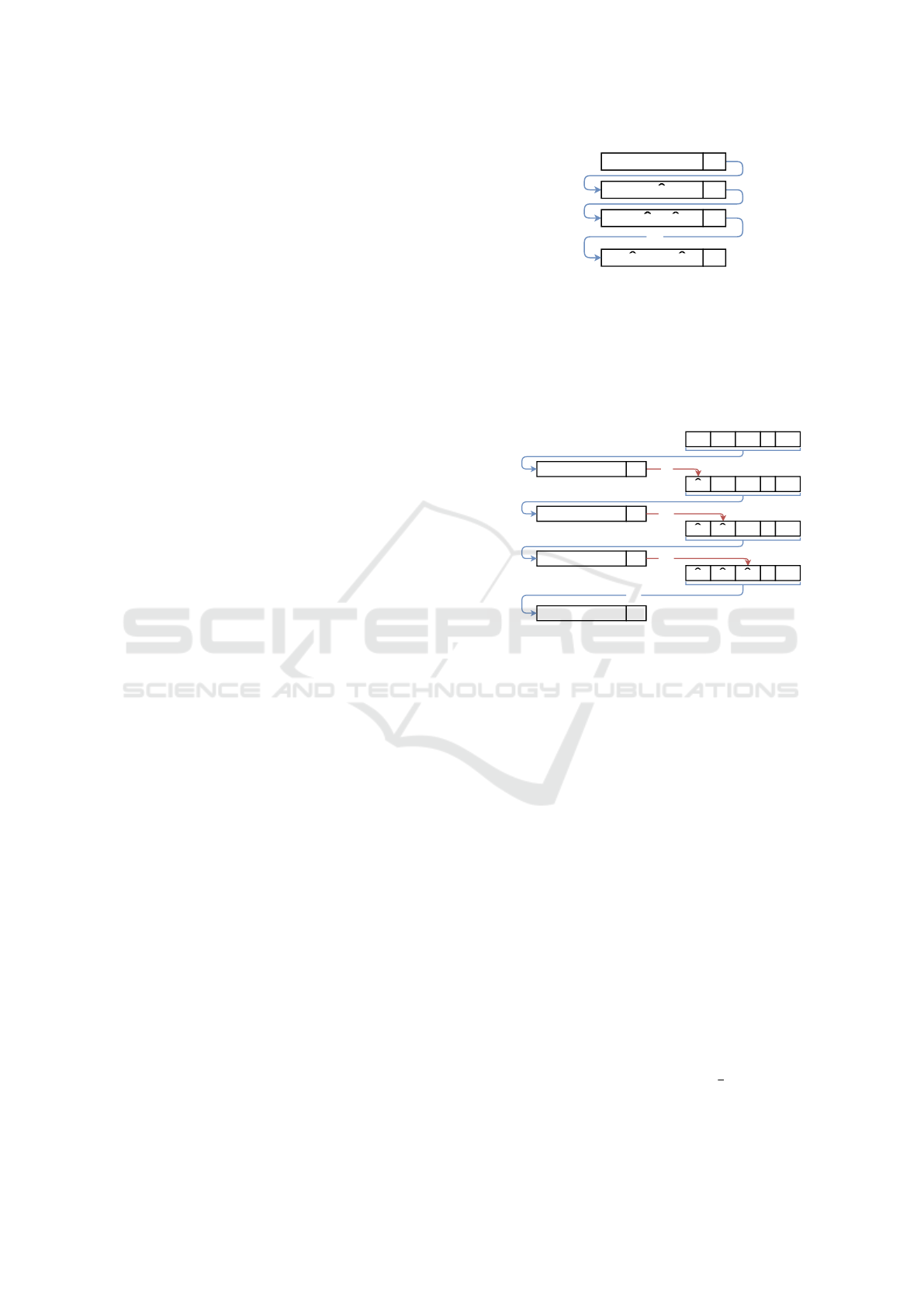
The performance of CC (which is shown in Fig-
ure 1) is as follows. Let us define T as the total time
required to build a binary model. First, a binary clas-
sifier that predicts the first label in the chain (λ
π1
)
given only the input features is built. Once this classi-
fier finishes, at t = T , a second classifier for following
label in the chain λ
π2
is built but now augmenting the
set of input features with the predictions of the previ-
ous label
ˆ
λ
π1
. At this moment, although λ
π1
was built
without considering the relationship with the rest of
labels, λ
π2
was predicted by a model being able to
model its relationship with λ
π1
. Then, a third classi-
fier including
ˆ
λ
π1
and
ˆ
λ
π2
as input features is built to
predict λ
π3
, and so on. Finally, the last classifier aims
to predict λ
πq
considering the predictions of the rest
of labels
ˆ
λ
π1
,· ·· ,
ˆ
λ
πq−1
. Therefore, considering an
ideal environment where all binary models required
the same runtime, the total time T
t
required by CC is
T
t
= qT .
Without modifying the definition of CC, we also
could see its operation as in Figure 2. In this case,
we have a structure that store the predictions of all la-
bels, called
ˆ
Y
Y
Y . Thus, each time that a binary classifier
is going to be built, all predictions that already exist
in this structure are included as input features. When
each classifier finishes its execution, it stores its pre-
dictions in the structure. For first classifier, as
ˆ
Y
Y
Y is
empty at t = 0, no predictions are included as input
x
λ
π1
x U λ
π1
λ
π2
x U λ
π1
U λ
π2
λ
π3
x U λ
π1
U ... U λ
πq-1
λ
πq
...
t=0
t=T
t=2T
t=(q-1)T
Figure 1: Operation of CC.
features. When the first classifier finishes at t = T ,
it stores
ˆ
λ
π1
in the structure, so the second classifier
could use them to predict λ
π2
, and so on. The opera-
tion of the method is the same as the previous one, but
we have included a structure that stores all the predic-
tions.
- - - -...
x U Ŷ
t=0
t = T
λ
π1
x U Ŷ
t=T
λ
π2
t=0
t=T
Ŷ
λ
π1
- - -...
t = 2T
x U Ŷ
t=2T
λ
π3
t=2T
λ
π1
λ
π2
- -...
t = 3T
x U Ŷ
t=(q-1)T
λ
πq
t=(q-1)T
λ
π1
λ
π2
λ
π3
-...
...
Figure 2: Other perspective of the operation of CC.
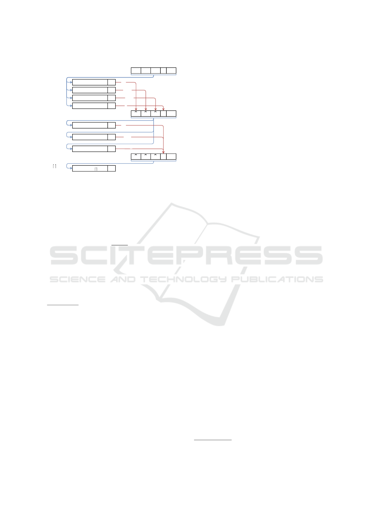
Therefore, we use this structure to define our pro-
posal Parallel Classifier Chains (PCC). In PCC, k bi-
nary classifiers are built in parallel. In Figure 3, the
operation of PCC for k = 4 is presented. In the begin-
ning, k binary classifiers to predict λ
π1
,· ·· , λ
πk
are
built without considering any relationship with the
rest of labels, only using input features (like the first
classifier in original CC). Then, each time that a clas-
sifier finishes, it stores its predictions in the structure
ˆ
Y
Y
Y , so next classifiers could use them as input features.
After including these predictions in the structure, a
new classifier for predicting next corresponding label
in the chain is built using all available predictions in
ˆ
Y
Y
Y . A new binary classifier is built each time in paral-
lel until all have been built. In the example, in t = T
the classifier to predict λ
π1
finishes and store its pre-
dictions; then a little time ε after, at t = T + ε the next
classifier (for λ
π5
) starts to be built. At t = T + ε
1
the
classifier for λ
π2
finishes, so it stores the predictions
and the next one (for λ
π6
) starts. Thus, the binary clas-
sifier for λ
π6
includes predictions of classifiers that
finished so far, i.e.,
ˆ
λ
π1
and
ˆ
λ
π2
. As a consequence
of building k binary classifiers in parallel, the ideally
expected total runtime of PCC is T
t
=
q
k
T .
This relaxed definition of PCC means that not as
many relationships are taken into account as in CC,
Speeding Up Classifier Chains in Multi-label Classification
31

- - - -...
x U Ŷ
t=0
t = T
λ
π1
t=0
Ŷ
x U Ŷ
t=0
t = T+ε
1
λ
π2
x U Ŷ
t=0
t = T+ε
2
λ
π3
x U Ŷ
t=0
...
λ
π4
λ
π1
λ
π2
λ
π3
-...
x U Ŷ
t=T
t=T+ε
x U Ŷ
t=T+ε1
x U Ŷ
t=T+ε2
λ
π1
λ
π2
λ
π3
-...
t=2T
t=2T+ε
...
λ
π5
λ
π6
λ
π7
x U Ŷ
t=(
-1
)T+ε
λ
πq
4
q
/
t=(
-1
)T+ε
4
q
/
...
Figure 3: Operation of PCC for k = 4.
but on the other hand, it is able to be built in parallel
using many threads. Note that in CC, the first clas-
sifier includes 0 labels as input features, the second
classifier includes 1 label as input feature, the third in-
cludes 2 labels, and finally, the last classifier includes
q − 1 labels as input features. Therefore, the average
number of labels included as input features for each
binary classifier in CC is
(q−1)∗q
2q
. On the other hand,
PCC is executed in parallel using k threads, the first k
classifiers include 0 labels as input features, and then,
the classifier k+1 includes 1 label as input feature, the
classifier k + 2 includes 2 labels, and so on, thus the
final classifier includes q − k labels as input features.
Therefore, in the case of PCC, the average number
of labels as input features in each of the classifiers is
(q−k)∗(q−k+1)
2q
. Furthermore, in cases where the label
space is very large, this difference could be negligible.
For example, for a dataset with 25 labels in the out-
put space, running PCC with k = 4 would reduce the
average number of labels used as input features up to
25% with respect to CC; however, for a dataset with
100 or 400 labels, PCC only reduces in 6% or 1% re-
spectively the average number of predicted labels as
features respect to CC.
Note that we are only parallelizing the training
phase of CC and not the testing one. The most
time-consuming part of running a classification algo-
rithm is the training phase (around 98% of the total
time (Roseberry and Cano, 2018), as shown below in
Section 4.2.1). Thus, we focused only on paralleliz-
ing the training phase instead of extending it also to
testing. The runtime of the test phase will depend so
much on the number of test examples, which could be
low in many real-world problems, so maybe on those
cases the process of making it parallel would consume
more time than sequential. Furthermore, note that by
parallelizing the test phase, we would be parallelizing
around 2% of the total runtime, so it would be practi-
cally negligible.
The aim of this paper is not only to speed up the
CC method but also to not harm its predictive perfor-
mance. Both the reduction in runtime and the varia-
tion in the predictive performance of CC are directly
related to the number of threads to execute in parallel
(k). For larger values of k, the runtime to build the
model would be lower but the final predictive perfor-
mance could be harmed. Moreover, the lack of some
labels to predict others may lead to removing noise
or unnecessary relationships, improving the perfor-
mance of CC.
Also, note that by reducing the runtime of CC, we
also reduce the runtime of the rest of methods based
on it, such as ECC. As aforementioned, ECC has been
proven to be one of the best methods in MLC, so
speeding it up would be a major contribution to the
scientific community.
4 EXPERIMENTAL STUDY
The aim of the experimental study is to evaluate the
effect produced by PCC in both the runtime and
the predictive performance. First, we describe the
datasets, evaluation metrics, and experimental set-
tings. Then, the results are presented and analyzed.
4.1 Experimental Setup
The experimental study has been carried out over a
wide set of 20 multi-label datasets
1
. A summary of
such datasets is shown in Table 1, including the num-
ber of examples (m), attributes (d), and labels (q).
These datasets have been selected according to the
number of labels, which ranges from simple datasets
with only 6 labels to datasets with a high complex la-
bel space with up to 400 labels. Furthermore, they
also include a wide range in both the number of ex-
amples (ranging from 225 to 43,910) and the number
of input attributes (ranging from 68 to 1,836).
We divided the experimental settings into two
parts, corresponding to the two main objectives of the
methodology: 1) Study of the runtime of PCC com-
pared to CC, and 2) Analysis of the predictive perfor-
mance of PCC. First, we aimed to prove that PCC sig-
nificantly reduces the time of CC to build the model;
however, we still aimed to not to harm the predictive
performance of the model. For this purpose, we ex-
ecuted PCC using different values for the number of
1
All the datasets are available at http://www.uco.es/
kdis/mllresources/
IoTBDS 2019 - 4th International Conference on Internet of Things, Big Data and Security
32

Table 1: Summary of datasets used in the experiments.
Dataset m d q
Stackex coffee 225 1,763 123
CAL500 502 68 174
Emotions 593 72 6
Birds 645 260 19
Genbase 662 1,186 27
PlantPseAAC 978 440 12
Medical 978 1,449 45
Langlog 1,460 1,004 75
Stackex chess 1,675 585 227
Enron 1,702 1,001 53
Yeast 2,417 103 14
Corel5k 5,000 499 374
Reuters-K500 6,000 500 103
Stackex chemistry 6,961 540 175
Bibtex 7,395 1,836 159
EukaryotePseAAC 7,766 440 22
Stackex cooking 10,490 577 400
Corel16k010 13,620 500 144
Ohsumed 13,930 1,002 23
Mediamill 43,910 120 101
threads, k = {2,4,8,12}. Furthermore, not only CC
was executed, but also BR, in order to have the base-
line where the relationships among labels are not con-
sidered at all.
In order to evaluate the MLC methods, many
widely used evaluation metrics in MLC have been se-
lected (Gibaja and Ventura, 2015). Hamming loss
(HL) is one of the most classic evaluation metrics
in MLC. It is a minimization metric that computes
the average number of times that a label is incor-
rectly predicted. HL is defined in Eq. 1 where ∆
stands for the symmetric difference among two bi-
nary sets
2
. Subset Accuracy (SA), also known as
exact match, is a very strict metric which requires
that for a given example, the multi-label prediction
exactly match the same as the true labels, including
both relevant and irrelevant labels. SA is defined in
Eq. 2 where JπK returns 1 if predicate π is true, and
0 otherwise. Moreover, F-Measure is a widely used
evaluation metric in traditional classification, and in
MLC it could be calculated from three different points
of view: Example-based F-Measure (ExF), Micro F-
Measure (MiF), and Macro F-Measure (MaF). ExF
computes the F-Measure for each example as in Eq. 3;
MiF first joins the confusion matrices of all labels and
then it computes F-Measure, as in Eq. 4 (let t p, f p,
and f n be the number of true positives, false posi-
tives, and false negatives); and finally, MaF computes
2
It is indicated with ↓ if it is a minimization metric or
with ↑ if it is maximization.
the F-Measure for each of the labels and then it aver-
ages the value as in Eq. 5. The main difference among
MiF and MaF is that the first gives more importance to
more frequent labels while the second gives the same
importance to all of them.
↓ HL =
1
m
m
∑
i=1
1
q
|y
y
y
i
∆
ˆ
y
y
y
i
| (1)
↑ SA =
1
m
m
∑
i=1
Jy
y
y
i
=
ˆ
y
y
y
i
K (2)
↑ ExF =
1
m
m
∑
i=1
2 ·
|
y
y
y
i
∩
ˆ
y
y
y
i
|
|
y
y
y
i
|
+
|
ˆ
y
y
y
i
|
(3)
↑ MiF =
∑
q
l=1
2 · t p
l
∑
q
l=1
2 · t p
l
+
∑
q
l=1
f n
l
+
∑
q
l=1
f p
l
(4)
↑ MaF =
1
q
q
∑
l=1
2 · t p
l
2 · t p
l
+ f n
l
+ f p
l
(5)
We executed the experiments over a random 5-
fold cross-validation procedure. Furthermore, both
CC and PCC were executed with 10 different values
for the seed for random numbers. Note that at each
execution, the chain is randomly selected. Finally, the
results of the different evaluation metrics were aver-
aged among the different executions, reporting both
the average value and the standard deviation.
Finally, in order to prove whether there exist sta-
tistical differences among the performance of the dif-
ferent methods, the Friedman’s test was conducted
first. Then, in cases where the Friedman’s test (Fried-
man, 1940) determined that there existed differences
among the methods, the Shaffer’s post-hoc test (Shaf-
fer, 1986) was also carried out to perform pairwise
comparisons. The adjusted p-values were reported,
since they consider the fact of performing multi-
ple comparisons without a significance level, provid-
ing more statistical information (Garcia and Herrera,
2008). It should be highlighted that all the experi-
ments have been performed on a machine with 6 Intel
Xeon E5646 CPUs at 2.40GHz and 24 GB of RAM.
PCC has been implemented using Mu-
lan (Tsoumakas et al., 2011b) and Weka (Hall
et al., 2009) frameworks, and the code is publicly
available in a GitHub repository
3
to facilitate the
openness and reproducibility of the results.
3
Source code available at https://github.com/
i02momuj/ParallelCC
Speeding Up Classifier Chains in Multi-label Classification
33

4.2 Experimental Results
In this section, we present the results of the differ-
ent experiments. First, we analyze the reduction in
runtime required by PCC to build a model compared
to CC. Secondly, we studied how the predictive per-
formance of PCC varies with respect to CC and BR.
Due to the great amount of results collected in the
experimental study, and in order to make the paper
more readable, only figures summarizing the results
are described in this paper. All the results, including
full tables with runtimes and evaluation metrics for
all methods, are available at the KDIS research group
website
4
.
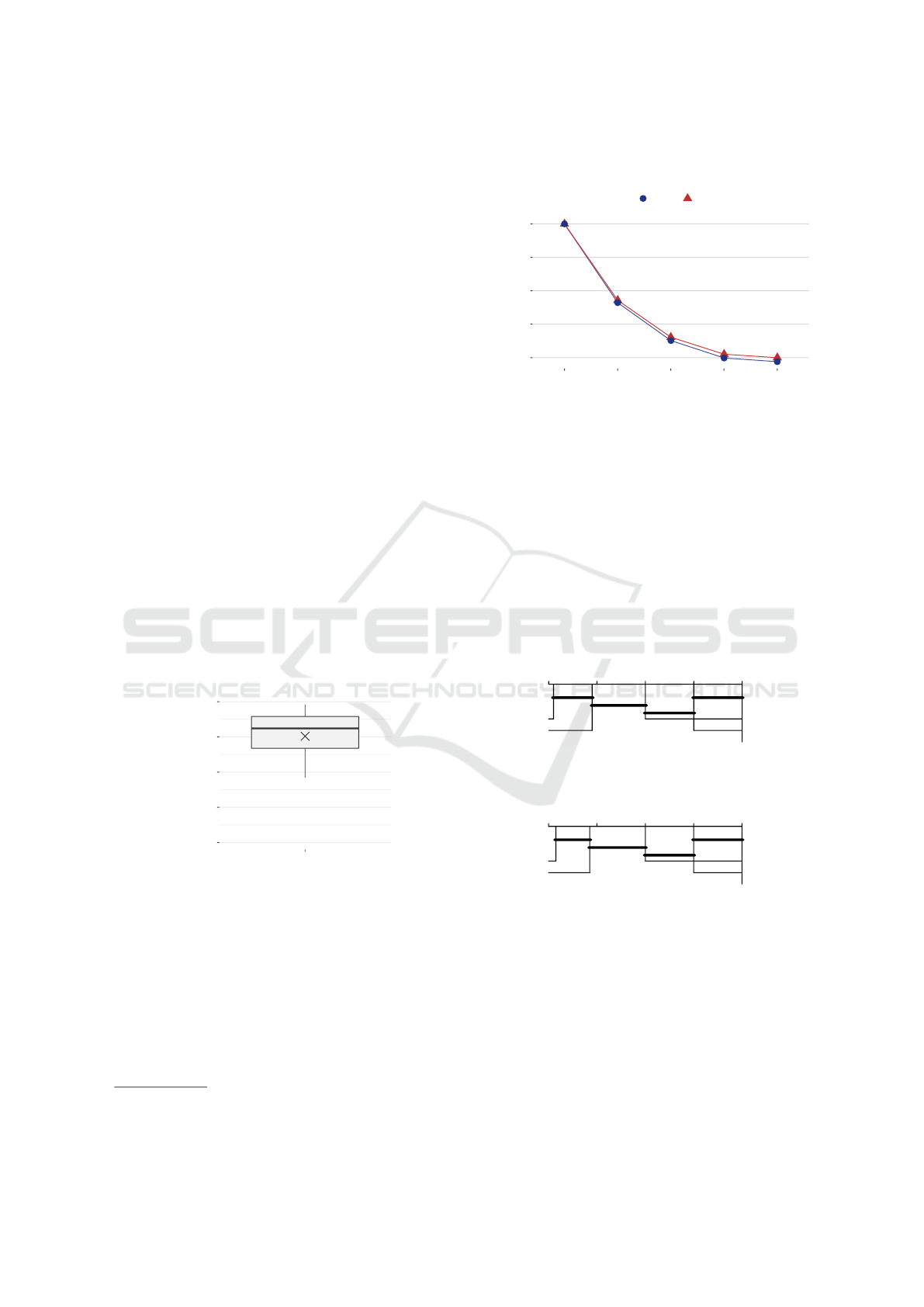
4.2.1 Analysis of the Runtime of PCC
In this first study we compare the runtime of PCC
with respect to CC. In this case, we differentiate be-
tween two different execution times: building runtime
(T
b
) and total runtime (T
t
). The former stands for the
time required to build the model, i.e., to learn from
the training data and build the classifier; while the lat-
ter stands for the total runtime to execute the algo-
rithm, including also the testing phase. However, and
as shown in Figure 4, the time spent in building a CC
is responsible of around 98% of the total runtime (on
average). Therefore, this fact supports the idea of only
parallelizing the building phase, since we are able to
run in parallel the most time-consuming part of CC.
0.90
0.92
0.95
0.98
1.00
Building time
Ratio of building time
in total time
Figure 4: Boxplot showing the percentage of time con-
sumed by building the method (T
b
) with respect to the total
runtime (T
t
).
Figure 5 shows how both T
t
and T
b
vary as
the number of threads for executing PCC in par-
allel becomes greater. The reduction of time re-
quired by PCC with respect to CC is calculated as
(time
PCC
− time
CC
)/ (time
CC
). Thus, negative values
stand for reduction of time. The obtained results were
as expected: for k = 2, T
b
was reduced over 47%; for
k = 4, T
b
was reduced over 70%; for k = 8, T
b
was
4
Detailed results available at http://www.uco.es/
kdis/ParallelCC/
reduced over 80%; and finally for k = 12, T
b
was re-
duced more than 82% on average for all datasets.
−0.8
−0.6
−0.4
−0.2
0.0
CC
Method
Variation in runtime
with respect to CC
Build Total
PCC
k=4
PCC
k=2
PCC
k=8
PCC
k=12
Figure 5: Variation of PCC runtime using different k values
with respect to CC.
Finally, as we showed that the runtime decreased
as expected when PCC was executed in parallel us-
ing more threads, we perform statistical comparisons
in order to determine if this reduction was significant.
The Friedman’s test determined that there were sta-
tistical differences in both T
t
and T
b
with adjusted
p-values of 3.33E − 16 and 4.44E − 16 respectively.
Thus, the Shaffer’s post-hoc test was also performed,
whose results are shown in Figures 6 and 7 for T
t
and
T
b
respectively, and using α = 0.01. In this case, we
prove that using more than k = 2 threads for PCC we
significantly reduced the runtime of CC.
1 2
3
4
5
CC
PCC
k=12
PCC
k=8
PCC
k=4
PCC
k=2
Figure 6: Results of Shaffer’s test for comparing total run-
time (T
t
) among CC and PCC using different values of k.
The test results were reported for α = 0.01.
1 2
3
4
5
CC
PCC
k=12
PCC
k=8
PCC
k=4
PCC
k=2
Figure 7: Results of Shaffer’s test for comparing building
runtime (T
b
) among CC and PCC using different values of
k. The test results were reported for α = 0.01.
4.2.2 Analysis of the Predictive Performance of
PCC
Once we have proven that the runtime of CC could be
significantly decreased with our proposal, we focused
on the predictive performance of PCC.
For this purpose, we first compared the pre-
dictive performance of PCC with different k val-
ues to the predictive performance of CC. In this
IoTBDS 2019 - 4th International Conference on Internet of Things, Big Data and Security
34

case, the variation in predictive performance of PCC
with respect to CC in terms of HL was calculated
as (HL
CC
− HL
PCC
)/ (HL
CC
). Furthermore, for SA
(and also for ExF, MiF, and MaF), as it is a max-
imization metric, the variation was calculated as
(SA
PCC
− SA
CC
)/ (SA
CC
). In all cases, negative val-
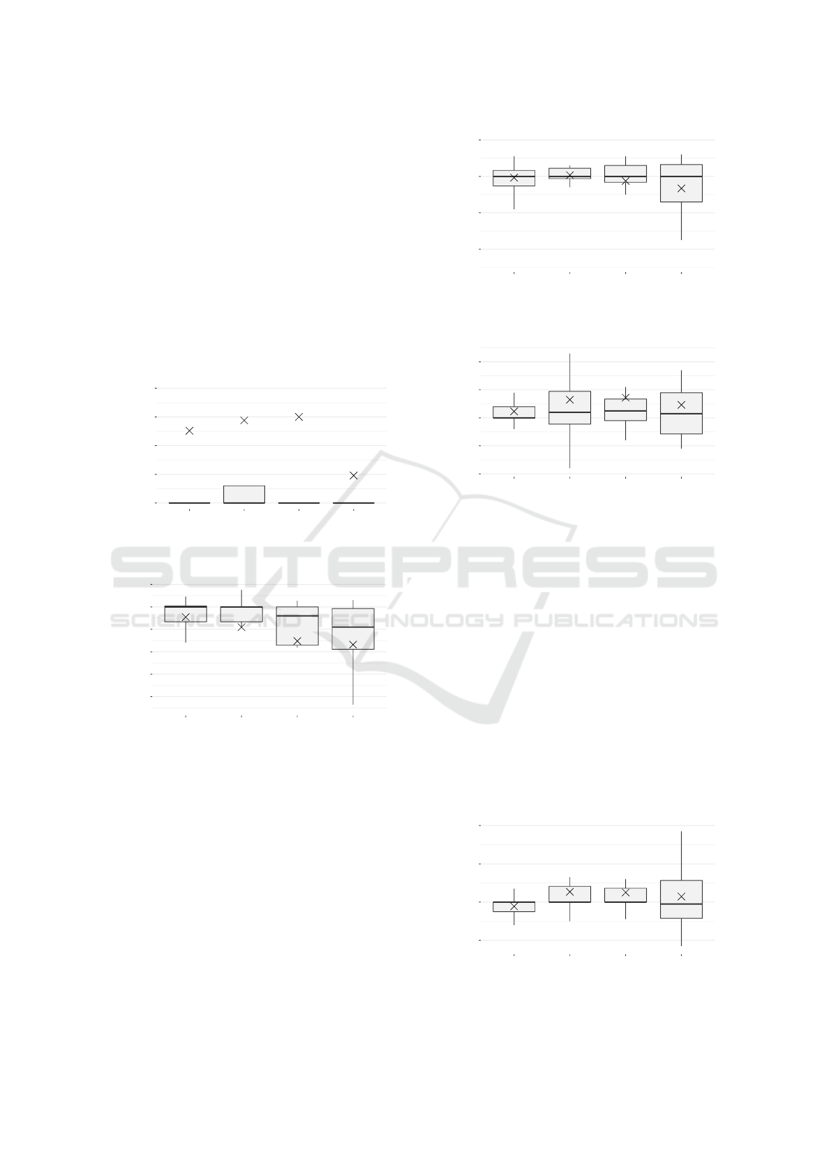
ues means a drop in the predictive performance. Fig-
ures 8, 9, 10, 11, and 12 show the boxplots with the
values of variation of the predictive performance of
PCC with respect to CC for HL, SA, ExF, MiF, and
MaF metrics, respectively. In all cases, outliers are
not represented for a better reading and understand-
ing of the figures. Moreover, the cross represents the
average value and the line inside the box indicates the
median value.
0.0000
0.0025
0.0050
0.0075
0.0100
PCC
Method
Variation in HL
k=2
PCC
k=4
PCC
k=8
PCC
k=12
Figure 8: Boxplots showing the variation in HL of PCC
using different values of k with respect to CC.
−0.20
−0.15
−0.10
−0.05
0.00
0.05
PCC
Method
Variation in SA
k=2
PCC
k=4
PCC
k=8
PCC
k=12
Figure 9: Boxplots showing the variation in SA of PCC us-
ing different values of k with respect to CC.
We observe that for HL, the median values of vari-
ation are near to 0 regardless of the value of k, so
although 12 binary models are built in parallel, the
median variation of HL still remains the same. Fur-
thermore, the average value of the change in HL is
over zero in all cases, which means that on average,
PCC outperforms CC in terms of HL regardless of the
degree of parallelization. In terms of SA, we could
see that the trend is to decrease the predictive perfor-
mance as the number of parallel threads is greater,
obtaining over an 8% drop in performance (on av-
erage) for k = 12. However, for lower k values, the
median value of variation with respect to CC is much
closer to zero. Similarly, ExF, MiF, and MaF exhibit
−0.04
−0.02
0.00
0.02
PCC
Method
Variation in ExF
k=2
PCC
k=4
PCC
k=8
PCC
k=12
Figure 10: Boxplots showing the variation in ExF of PCC
using different values of k with respect to CC.
−0.02
−0.01
0.00
0.01
0.02
PCC
Method
Variation in MiF
k=2
PCC
k=4
PCC
k=8
PCC
k=12
Figure 11: Boxplots showing the variation in MiF of PCC
using different values of k with respect to CC.
a similar behavior. The median value of variation is
near zero in all cases; nevertheless, the trend in these
metrics, on average, is to even improve the perfor-
mance of CC (except for higher parallelization for
ExF). This could be given by the fact that PCC con-
siders the relationships among labels but in a more
relaxed way than CC (also related to k), so maybe
in some cases it could lose useful information, but in
other cases PCC removes noise or useless informa-
tion that leads to a slightly better performance. Note
that SA is such a strict metric, that maybe the perfor-
mance in SA decreases because a lower percentage of
examples are perfectly predicted but it still maintains
the same performance on average on other more rep-
resentative evaluation metrics such as F-Measure.
−0.02
0.00
0.02
0.04
PCC
Method
Variation in MaF
k=2
PCC
k=4
PCC
k=8
PCC
k=12
Figure 12: Boxplots showing the variation in MaF of PCC
using different values of k with respect to CC.
Speeding Up Classifier Chains in Multi-label Classification
35

Finally, the performance of PCC was not only
compared to CC but also to BR. As our proposal
removes some of the links among binary methods
from CC (i.e., does not consider as many relationships
among labels as CC does), we also wanted to include
in this comparison BR as a baseline method that does
not consider relationships among labels at all.
We performed statistical tests in order to deter-
mine whether there are significant differences in the
performance of these algorithms. First, we performed
the Friedman’s test, which concluded that there were
not statistical differences among the different meth-
ods in HL, ExF, and MiF at 99% confidence (with
p-values 3.20E − 2, 1.04E − 1, and 1.34E − 1 respec-
tively). On the other hand, it was determined that for
SA and MaF, there were statistical differences in the
performance of the different methods, with p-values
7.35E − 3 and 8.04E − 3 respectively. For these two
metrics, we performed the Shaffer’s test too, whose
results are presented in Figures 13 and 14 for SA and
MaF respectively, and α = 0.01.
Although Friedman’s test stated that for SA there
were statistical differences in the performance of the
algorithms, the Shaffer’s post-hoc test determined that
there were not. On the other hand, for MaF, Shaffer’s
test stated that BR significantly outperformed PCC
using k = 2 and k = 12; however, no significant dif-
ferences were found among CC and PCC.
2
3
4
5
CC BR
PCC
k=2
PCC
k=4
PCC
k=12
PCC
k=8
Figure 13: Results of Shaffer’s test for comparing SA
among BR, CC and PCC using different values of k. The
test results were reported for α = 0.01.
2
3
4
5
BR CC
PCC
k=4
PCC
k=8
PCC
k=2
PCC
k=12
Figure 14: Results of Shaffer’s test for comparing MaF
among BR, CC and PCC using different values of k. The
test results were reported for α = 0.01.
Consequently, at this point we demonstrated that
there were no significant differences between CC and
PCC in terms of predictive performance, even when it
was executed in parallel in a high number of threads.
Only for one metric, PCC with k = 2 and k = 12
performed significantly worse than BR at 99% confi-
dence. Therefore, we reached the objective of this pa-
per, to significantly reduce the runtime to build a CC
model without significantly harming its performance.
5 CONCLUSIONS
In this paper we have proposed a modified version of
Classifier Chains (CC) for multi-label classification,
called Parallel Classifier Chains (PCC). Unlike CC,
PCC is able to build each binary model in parallel us-
ing k threads, allowing to speed up the required run-
time to build the whole MLC model.
The experiments confirmed that PCC was able
to significantly reduce the runtime needed by CC to
build a model, reducing the runtime over 47% when
executing in 2 threads, and up to 80% when using 8
threads. Furthermore, the fact of considering the re-
lationship among labels in a more relaxed way than
CC could led PCC to lose useful information; how-
ever, PCC also got rid of useless information and
noise when modeling a given label, tending to im-
prove its performance in most metrics as the paral-
lelization was higher. All these results were validated
using non-parametric statistical analysis at 99% confi-
dence. These results confirmed that the predictive per-
formance of PCC and CC was statistically the same,
but the runtime was drastically reduced.
For future work, we plan to investigate further par-
allel models that also take into account the relation-
ships among labels, especially in the context of high-
dimensional and imbalanced label spaces.
ACKNOWLEDGEMENTS
This research was supported by the Spanish Min-
istry of Economy and Competitiveness and the Euro-
pean Regional Development Fund, project TIN2017-
83445-P. This research was also supported by the
Spanish Ministry of Education under FPU Grant
FPU15/02948.
REFERENCES
Babbar, R. and Sch
¨
olkopf, B. (2017). Dismec: Distributed
sparse machines for extreme multi-label classification.
In ACM International Conference on Web Search and
Data Mining, pages 721–729.
Brandt, P., Moodley, D., Pillay, A. W., Seebregts, C. J., and
de Oliveira, T. (2014). An Investigation of Classifica-
tion Algorithms for Predicting HIV Drug Resistance
without Genotype Resistance Testing, pages 236–253.
Charte, F., Rivera, A. J., del Jesus, M. J., and Herrera, F.
(2014). Li-mlc: A label inference methodology for
addressing high dimensionality in the label space for
multilabel classification. IEEE Transactions on Neu-
ral Networks and Learning Systems, 25(10):1842–
1854.
IoTBDS 2019 - 4th International Conference on Internet of Things, Big Data and Security
36

Dembczynski, K., Cheng, W., and H
¨
ullermeier, E. (2010).
Bayes optimal multilabel classification via probabilis-
tic classifier chains. In International Conference
on International Conference on Machine Learning,
pages 279–286.
Friedman, M. (1940). A comparison of alternative tests of
significance for the problem of m rankings. Annals of
Mathematical Statistics, 11(1):86–92.
Garcia, S. and Herrera, F. (2008). An extension on “sta-
tistical comparisons of classifiers over multiple data
sets” for all pairwise comparisons. Journal of Ma-
chine Learning Research, 9:2677–2694.
Gibaja, E. and Ventura, S. (2014). Multi-label learning: a
review of the state of the art and ongoing research.
Wiley Interdisciplinary Reviews: Data Mining and
Knowledge Discovery, 4(6):411–444.
Gibaja, E. and Ventura, S. (2015). A tutorial on multilabel
learning. ACM Computing Surveys, 47(3):52:1–52:38.
Goncalves, E., Plastino, A., and Freitas, A. A. (2015). Sim-
pler is better: a novel genetic algorithm to induce com-
pact multi-label chain classifiers. In Conference on
Genetic and Evolutionary Computation Conference,
pages 559–566.
Gonzalez-Lopez, J., Cano, A., and Ventura, S. (2017).
Large-scale multi-label ensemble learning on spark.
In IEEE Trustcom/BigDataSE/ICESS, pages 893–900.
Gonzalez-Lopez, J., Ventura, S., and Cano, A. (2018). Dis-
tributed nearest neighbor classification for large-scale
multi-label data on spark. Future Generation Com-
puter Systems, 87:66 – 82.
Hall, M., Frank, E., Holmes, G., Pfahringer, B., Reutemann,
P., and Witten, I. H. (2009). The weka data mining
software: An update. ACM SIGKDD Explorations
Newsletter, 11(1):10–18.
Hsu, D. J., Kakade, S. M., Langford, J., and Zhang, T.
(2009). Multi-label prediction via compressed sens-
ing. In International Conference on Neural Informa-
tion Processing Systems, pages 772–780.
Melki, G., Cano, A., Kecman, V., and Ventura, S. (2017).
Multi-target support vector regression via correlation
regressor chains. Information Sciences, 415-416:53–
69.
Moyano, J. M., Gibaja, E., and Ventura, S. (2017). An
evolutionary algorithm for optimizing the target or-
dering in ensemble of regressor chains. In 2017 IEEE
Congress on Evolutionary Computation (CEC), pages
2015–2021.
Moyano, J. M., Gibaja, E. L., Cios, K. J., and Ventura, S.
(2018). Review of ensembles of multi-label classi-
fiers: Models, experimental study and prospects. In-
formation Fusion, 44:33 – 45.
Nasierding, G. and Kouzani, A. (2010). Image to text trans-
lation by multi-label classification. In Advanced In-
telligent Computing Theories and Applications with
Aspects of Artificial Intelligence, volume 6216, pages
247–254.
Prabhu, Y. and Varma, M. (2014). Fastxml: A fast, accurate
and stable tree-classifier for extreme multi-label learn-
ing. In ACM SIGKDD International Conference on
Knowledge Discovery and Data Mining, pages 263–
272.
Read, J. (2008). A pruned problem transformation method
for multi-label classification. In Proceedings of the
NZ Computer Science Research Student Conference,
pages 143–150.
Read, J., Pfahringer, B., Holmes, G., and Frank, E. (2011).
Classifier chains for multi-label classification. Ma-
chine Learning, 85(3):335–359.
Roseberry, M. and Cano, A. (2018). Multi-label kNN
Classifier with Self Adjusting Memory for Drifting
Data Streams. In International Workshop on Learning
with Imbalanced Domains: Theory and Applications,
ECML-PKDD, pages 23–37.
Shaffer, J. P. (1986). Modified sequentially rejective multi-
ple test procedures. Journal of the American Statisti-
cal Association, 81(395):826–831.
Skryjomski, P., Krawczyk, B., and Cano, A. (2018). Speed-
ing up k-Nearest Neighbors Classifier for Large-Scale
Multi-Label Learning on GPUs. Neurocomputing, In
press.
Tang, L. and Liu, H. (2009). Scalable learning of collective
behavior based on sparse social dimensions. In ACM
Conference on Information and Knowledge Manage-
ment, pages 1107–1116.
Tsoumakas, G. and Katakis, I. (2007). Multi-label classi-
fication: An overview. International Journal of Data
Warehousing and Mining, 3(3):1–13.
Tsoumakas, G., Katakis, I., and Vlahavas, I. (2008). Effec-
tive and efficient multilabel classification in domains
with large number of labels. In Workshop on Mining
Multidimensional Data, ECML-PKDD.
Tsoumakas, G., Katakis, I., and Vlahavas, I. (2010). Data
Mining and Knowledge Discovery Handbook, Part
6, chapter Mining Multi-label Data, pages 667–685.
Springer.
Tsoumakas, G., Katakis, I., and Vlahavas, I. (2011a). Ran-
dom k-labelsets for multi-label classification. IEEE
Transactions on Knowledge and Data Engineering,
23(7):1079–1089.
Tsoumakas, G., Spyromitros-Xioufis, E., Vilcek, J., and
Vlahavas, I. (2011b). Mulan: A java library for
multi-label learning. Journal of Machine Learning
Research, 12:2411–2414.
Speeding Up Classifier Chains in Multi-label Classification
37