
Ensembled Outlier Detection using Multi-Variable Correlation in
WSN through Unsupervised Learning Techniques
Marc Roig, Marisa Catalan and Bernat Gastón
Fundació Privada I2CAT, Gran Capità 2-4, Barcelona, Spain
Keywords: Internet of Things, Wireless Sensor Networks, Machine Learning, Outlier Detection, Big Data, Unsupervised
Learning.
Abstract: Outlier detection in Wireless Sensor Networks is a crucial aspect in IoT, since cheap sensors tend to be
seriously exposed to errors and inaccuracies. Hence, there is the need of a solution to improve the quality of
the data without increasing the cost of the sensors. In Big Data paradigms, it is difficult to exploit the temporal
correlation of sensors since Big Data architectures and technologies do not process data in order. In this paper,
a complete study of multi-variable based outlier detection is carried out. Firstly, three known unsupervised
algorithms are analysed (Elliptic Envelope, Isolation Forest and Local Outlier Factor) and are tested in a big
data architecture. Secondly, an ensemble outlier detector (EOD) is created with the outputs of these algorithms
and it is compared, in a Lab environment, with previous results for different parameters of contamination of
the training set. The analysis of the results show that for correlated variables, multi-variable EOD has a very
good detection rate with a very low false alarm rate. Finally, the EOD is used in a real world scenario in the
city of Barcelona and the results are analysed using spectral-decomposition techniques which indicate that
EOD has a good performance in a real case.
1 INTRODUCTION
The decrease in the cost of sensors in these last years
is one of the reasons that has promoted the adoption
of the Internet of Things (IoT) paradigm in many
sectors and domains. From Smart Cities to Industry
4.0, IHealth or Autonomous Guided Vehicles
(AGVs), to name just a few, the inclusion of low price
sensors has allowed companies to improve their
competitiveness and create new business models.
Hence, sensors are on the basis of the value’s
pyramid of nearly any company willing to digitalize
and improve their products and processes. However,
sensors do not add value by themselves. The data that
they produce is the one that, once analysed and/or
visualized, can provide value to the users. Data with
low quality (i.e. with many errors) is difficult to be
analysed and it may lead to incorrect assumptions or
decisions. Moreover, in Big Data environments it is
impossible to find and neutralize these errors
manually.
Consequences of bad data quality can cause major
impacts on applications, for example, bad
measurements on Intensive Care Unit (ICU) patients,
an error in an automated manufacturing chain or a
mismeasurement in a modern smart city, where
public policies are decided depending on the data
reported by the sensors (e.g. banning the use of
pollutant cars when the levels of pollution are
considered dangerous).
In general, we can conclude that any sensor is as
good as the data that it provides. It has been shown
empirically that sensors (especially cheap ones) are
seriously affected by several sources or errors such as
noise, inaccuracies and impression, hardware
problems, and low voltage to name just a few
(Elnahawy and Natch, 2003). In many applications,
using high quality sensors that reduce errors may not
be an option due to their high cost. However, it is
possible to apply software based outlier detection
techniques to the collected data in order to identify
erroneous samples and improve the quality of the
resulting data.
There have been many research efforts in outlier
detection in the field of Wireless Sensor Networks
(WSNs) where limited resources, frequent physical
failures and exposition to attacks are the main factors
to consider.
In (Shikha Shukla et al. 2014), authors perform a
complete survey of the different techniques of outlier
38
Roig, M., Catalan, M. and Gastón, B.
Ensembled Outlier Detection using Multi-Variable Correlation in WSN through Unsupervised Learning Techniques.
DOI: 10.5220/0007657400380048
In Proceedings of the 4th International Conference on Internet of Things, Big Data and Security (IoTBDS 2019), pages 38-48
ISBN: 978-989-758-369-8
Copyright
c
2019 by SCITEPRESS – Science and Technology Publications, Lda. All rights reserved

detection in WSNs, classifying them between
Statistical-Based approaches, Nearest Neighbour
approaches, Cluster-Based approaches,
Classification-Based approaches and Spectral
Decomposition-Based approaches.
Cluster-based approaches in IoT have several
advantages over the rest of techniques. Firstly, even
if supervised systems (mainly Classification-based
approaches) are commonly used for calibration of
sensors (Spinelle et al., 2015) and (Pena et al., 2003),
it is difficult to create supervised systems in a real
world IoT scenario, because they do not adapt to new
conditions (e.g. a change of location of the sensor)
easily. Secondly, statistical approaches suffer from
the adaption to real time and to the Big Data paradigm
associated with IoT. Thirdly, unsupervised systems
can be combined with spectral decomposition-based
approaches since these are focused on variable
reduction (usually for visualization, even if there has
been research on spectral decomposition-based
outlier detection using PCA techniques (Ghorbel et
al., 2015) and (Zheng et al., 2018). Finally,
unsupervised cluster-based systems do not need to
know the number of clusters in advance.
In general, unsupervised clustering techniques
have the advantage that they model the “usual”
behaviour of the system and then, they detect any
anomaly out of this behaviour. This is exactly the
problem to be solved by outlier detection in sensor
networks. Moreover, one may note that outlier
detection techniques can be combined with
supervised learning techniques in a way that these
anomalies can be classified in different classes
(different types of anomalies or events).
Most of the work related to outlier detection in
WSN have been focused on exploiting the temporal
(time sequenced) and spatial (location) correlation of
the different sensors measurements (Zheng et al.,
2018) and (Yang et al., 2008) with distributed
approaches focusing also on multi-variable as a
secondary correlation (Barakkath Nisha et al., 2014).
All these techniques are usually evaluated using a
clean dataset where outliers are added artificially,
since a labelled dataset is needed to evaluate an
algorithm and it is difficult to obtain such dataset
from real measurements.
In the paradigm of Big Data introduced by the
MapReduce (Dean and Ghemawat, 2008) technique
implemented in the most known technologies in the
field like Hadoop (Shvachko et al., 2010) or Spark
(Zaharia et al., 2016), data is not processed in
temporal order. Instead of that, chunks of data are
distributed to several nodes and MapReduce tasks are
launched in parallel. Hence, it is difficult to base an
outlier analysis in time correlations using a Big Data
approach.
Moreover, according to our knowledge, there is
no study that evaluates the multi-variable correlation
separately from the temporal and spatial correlations.
This would be useful in order to show the
characteristics of outlier detection for each one of
these correlations (temporal, spatial, multi-variable)
separately.
Finally, in real world IoT scenarios, most of the
variables are correlated, like the temperature and
vibration of a machine in a manufacturing line or the
different pollutant agents in a smart city
Hence, in this paper we aim to exploit and
evaluate the multi-variable correlation in outlier
detection. Firstly, to detect these outliers we use a set
of three well-known unsupervised algorithms,
namely Elliptic envelope, Isolation Forest and Local
Outlier Factor (Section 2). With their outputs, we
build an Ensemble Outlier Detector (EOD) based on
a majority voting system.
Secondly, we perform this analysis using the well-
known and broadly used Intel Berkeley dataset (Intel
Berkeley Research Lab, 2004) (Section 3). We
evaluate this system using the standard evaluation
techniques based on Detection Rate (DR) and False
Alarm Rate (FAR) with artificially generated outliers
composed of local and global outliers.
Thirdly, we evaluate the proposed model in a real
case scenario in the city of Barcelona, within the
scope of the GrowSmarter project (Growsmarter
project, 2019), using the data provided by a cluster of
sensors of 16 variables installed in bikes that move
around the city (Section 4).
Finally, we present future evolutions of the EOD
and we expose the conclusions (Section 5).
2 ENSEMBLE OUTLIER
DETECTOR
Ensemble methods are widely used to increase the
accuracy of the predictions when different criteria
need to be applied for decision making using data-
driven systems. For example, Skyline is a popular
open source project which uses ensemble methods for
outlier detection in time-series data (Stanway, 2013).
This work takes advantage of very well-known
unsupervised techniques for outlier detection in order
to get a unique robust classification.
In the presented Ensemble Outlier Detector, the
first implemented technique is Elliptic Envelope (EE)
(Rousseeuw and Van Driessen, 1999), which is based
Ensembled Outlier Detection using Multi-Variable Correlation in WSN through Unsupervised Learning Techniques
39
on the minimum covariance determinant (MCD) as a
robust estimator for a given multivariate space. It
generates an elliptical space around the centre of mass
of the data using the covariance matrix of the features.
Given these decision boundaries, any point outside
the space is tagged as an abnormal point.
The second unsupervised algorithm is Isolation
Forest (IF) (Liu et al., 2008), a method that uses
multiple random trees to find the conditions that
isolate abnormal values. Based on the assumption that
an outlier can be easily isolated from the other data
points, it generates multiple random conditions that
split the data between greater and smaller values. The
shorter the number of conditions needed to isolate a
sample are, the higher is the probability of that
specific sample to be an outlier.
The last one is the Local Outlier Factor (LOF)
(Breunig et al., 2000). It is a density-based outlier
detection method that uses k-nearest neighbour’s
algorithm (KNN) to find local outliers. Using relative
density of a sample against its neighbours, the
algorithm is able to find abnormal points. In contrast
to proximity-based clustering, LOF is able to detect
local outliers inside the data distribution.
Finally, the proposed method is an Ensemble
Outlier Detector (EOD). This system takes advantage
of the three different techniques (EE, IF and LOF) to
have a robust binary classification indicating if a
sample is an outlier or not. Our outlier detector model
is described as follows. Firstly, the training is done in
each of the three algorithms using a representative
subset of the sensor data. Secondly, the sensor records
are introduced in the model and classified by each of
the three algorithms. Finally, the EOD determines the
final classification. The vote system delivers whether
or not the sample is an outlier and isolates all the
abnormal values from the normal values.
A record is detected as an outlier depending on
how many times the internal algorithms classified it
as an abnormal value. Taking into account that an
outlier classification from one algorithm means a
positive vote (+1) and a normal from one algorithm
classification means abstention (0), the vote system
applied on a sample point p through the three internal
algorithms of the EOD is defined as:
(1)
3 RESULTS
In this section the outlier detection will be executed
and evaluated using the Intel Berkeley database (Intel
Berkeley Research Lab, 2004). The dataset comprises
samples from fifty-one sensors distributed across a
controlled laboratory during the timeframe between
February 28th and April 5th, 2004. There are 2.3M
samples overall with each sensor sampling every
thirty-one seconds. For each sensor we have its
coordinates (location in the room), and for each
sample we have the timestamp, the temperature (in
Cº), the humidity (relative from 0% to 100%), the
light (in LUX) and the voltage (in Volts).
In order to evaluate the performance of the
algorithms and for simplicity, we consider only the
temperature and the humidity for two reasons.
Firstly, because we know that there exist a correlation
between them and our method is precisely based on
multi-variable correlation. Hence, it only makes sense
with correlated variables. Secondly, because it is
much easier to show the data graphically in two
dimensions without the need to use spectral-
decomposition techniques. Later on, we will be able
to compare our results over this dataset with the
results in the real scenario graphically (Section 4),
since without labelled datasets we will be unable to
provide more accurate metrics.
Over the selected subset of data of the Intel
dataset, synthetic outliers are created. This is a
commonly used procedure for comparing outlier
detection techniques in WSN (Ghorbel et al., 2015),
(Zheng et al., 2018) and (Yang et al., 2008).
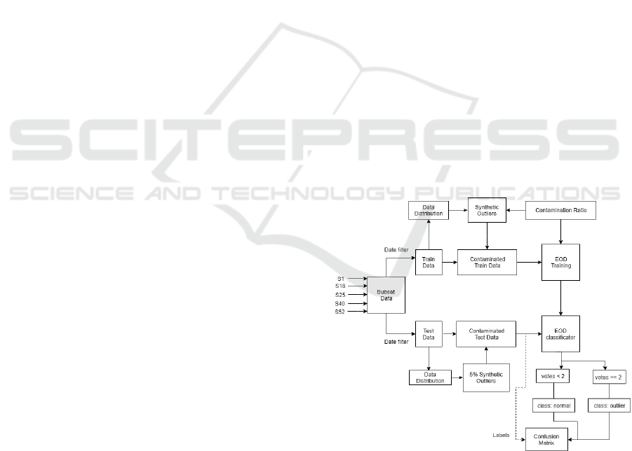
Figure 1: Evaluation diagram.
In Figure 1 the main workflow of the evaluation
method is shown. The first step is to select a suitable
subset of sensors to build our training space. Five
node sensors are chosen as a representative subset of
the whole sensor deployment, specifically S1, S18,
IoTBDS 2019 - 4th International Conference on Internet of Things, Big Data and Security
40
S25, S40 and S52. From these five sensors, a time
period of 3 working days is selected as being a
representative set of samples, specifically from
2015/03/04 until 2015/03/06. At this stage, the train
subset can be studied to make sure that there are not
abnormal values. Once we know that all the values
are reliable, the next step is to mix synthetic outliers
using random SciPy NumPy library (Jones et al.
2018). The percentage of synthetic outliers over the
training dataset is called the contamination c and it is
an important parameter for algorithm training.
A synthetic outlier O is created as random value
inside a Gaussian distribution with a constant value
deviated a 30% from the minimum or the maximum
measure of a variable var with mean and variance
. The formula is randomly selected for every new O
to make sure that outliers are created above the
maximum and below the minimum of the data
distribution. See formula details below:
(2)
(3)
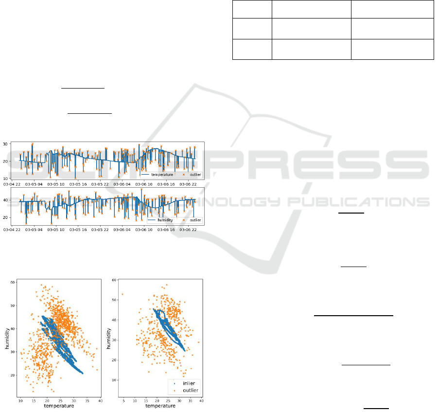
Figure 2: Train set time series of sensor 1 for temperature
(top) and humidity (down) with 5% of outliers.
Figure 3: Train (left) and test (right) data correlation for
c=5%.
In Figure 2, the data of one sensor over the three
training days is shown graphically for both,
temperature and humidity. The crosses are the
synthetic outliers. The correlation of both variables
with the outliers is shown in Figure 3, where it can be
seen that the outliers are generated trying not to be too
obvious for the algorithms and containing both, local
outliers (outlier in one variable) and global outliers
(outliers in both variables).
The classification output (predictions) of our
EOD will be compared to the real class input (labels)
in order to generate the confusion matrix (Table 1).
Table 1: Confusion Matrix.
Predicted Outlier
Predicted Normal
Real
Outlier
True Positive (TP)
False Negative (FN)
Real
Normal
False Positive (FP)
True Negative (TN)
Finally, some calculations will be done on top of
the confusion matrix to discuss the results. To do so,
very well-known metrics as False Alarm Rate (FAR),
Detection Rate (DR) and accuracy (ACC) will be
useful. In addition, other interesting metrics will be
computed to give a better understanding of the results.
In these experiments, F1-score will be a good
indicator of the compromise between DR and
precision.
The detection rate is:
(4)
The false alarm rate is:
(5)
The accuracy is:
(6)
Finally, the F1-score is:
(7)
With
(8)
Outlier detection techniques are expected to have
high DR while maintaining low FAR. ACC is
required to be high as it shows the successful
Ensembled Outlier Detection using Multi-Variable Correlation in WSN through Unsupervised Learning Techniques
41
predictions in front of to the total number of samples.
Similarly, a high f1-score means a good trade-off
between correct predictions and misclassifications.
Furthermore, ROC curves are used to evaluate the
compromise between DR and FAR.
Knowing the contamination ratio of our train data,
the system can be fitted using the contaminated train
set and the contamination ratio. After the training step
is done, the system is ready to classify new data that
it had never seen before. In the same way that we did
with the training set, we will consider the next day
(2015/03/07) as a clean test set to impute synthetic
outliers on it. The chosen outlier ratio in the testing
set is the 5% of the data. Finally, the system will
detect if a sample is or is not an outlier and this
prediction will be compared to the original label. To
do all these computations we have implemented our
algorithms using Python and launching them using
Spark (through the PySpark library). Our method is
completely in line with the Big Data paradigm and its
100% parallelizable using MapReduce techniques.
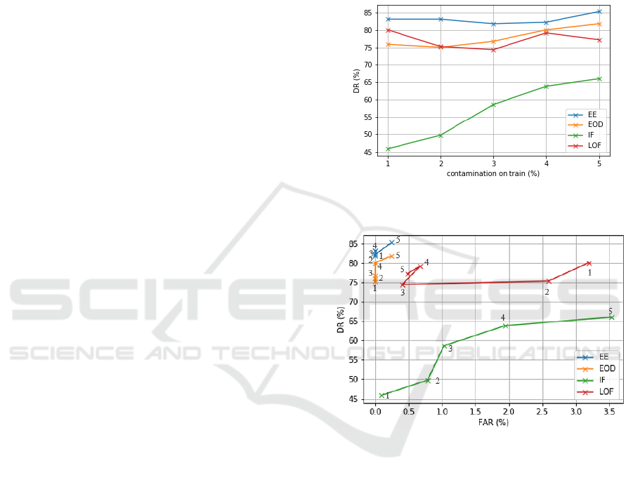
We propose five experiments to evaluate the
efficiency of the different algorithms. The
contamination on train goes from 1% to 5% in steps
on 1 %. The objective is to evaluate the effect of the
training contamination parameter applied to same test
set. The results are shown in Figure 4, where the DR
of the different methods is presented for the five
different experiments. Firstly, LOF performance is
good for low contamination training rate while IF has
very poor DR. Secondly, the performance of LOF
slightly decreases as the contamination in training
increases. Finally, except for LOF, the trend suggests
that DR increases with the contamination on the train
data. This effect is due to the need of the algorithms
to create robust decision spaces while training;
something that cannot be achieved with a very low
contamination.
In Figure 5, the trade-offs between the resulting
DR and FAR for the five experiments are shown.
Each point represents a different contaminated
training set (with the numbers indicating the
contamination ratio). As we have seen before, LOF is
able to obtain very good DR for low contaminated
train sets, but the FAR it’s also very high compared
to the other methods. In contrast, the FAR of EE
remains zero for low contaminated experiments.
Although IF has its better performance for
contamination equal 4%, its DR and FAR are still
poor in comparison to the other methods. In
summary, EE, LOF and IF have their best
performances for c = 4%.
According to these metrics, we can conclude that
EE is the algorithm with better results. The main
reason is that the simplicity of the analysed dataset (2
variables) and the distribution of these two variables
(Figure 3) fit perfectly in the elliptic shape of EE. In
contrast IF performs the worst by difference for the
same reason, since having only two variables does not
allow IF to isolate easily the outliers in the forest that
it creates. Finally, LoF is between both results, being
able to achieve a good accuracy but with a high FAR.
Figure 4: DR evolution over the increase of the train
contamination percentage.
Figure 5: DR - FAR trade-off shown by the three algorithms
for the five tests.
From these results, we can extract two main
conclusions. Firstly, that the scenario chosen benefits
EE while it detriments both IF and LoF. IF needs
more variables to increase its performance while LoF
needs also a more complex scenario to be able to
leverage its capabilities in finding local outliers. We
think that with a more complex scenario like the one
proposed in the real case (Section 4) the performance
of the three algorithms would be closer. Secondly, we
conclude that our constructed EOD works very well
even in this scenario with heterogeneous results, with
EOD being very close to EE in performance. We
think that with a more balanced scenario, the EOD
can easily be the best in terms of performance.
In order to have a better understanding of the
behaviour of our EOD, a deeper analysis on results is
5
IoTBDS 2019 - 4th International Conference on Internet of Things, Big Data and Security
42
needed. For the sake of clarity, a static train
contamination is needed. The next experiments are
done with a 5 % contaminated training and test
datasets.
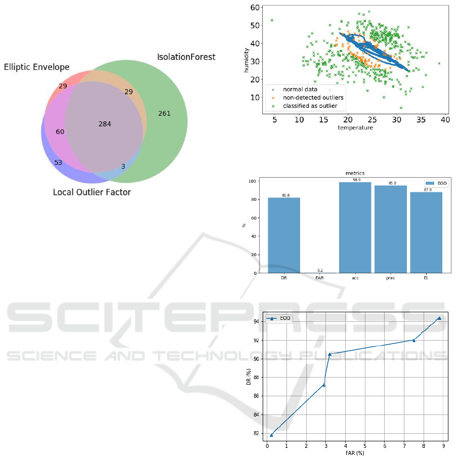
Figure 6: Venn diagram of the outliers detected by each one
of the three algorithms.
The first question to answer is how the algorithms are
contributing to the EOD. In Figure 6, the Venn
diagram shows the intersection between the outliers
detected by each one of the algorithms. Due to the
EOD nature, only the outliers detected by two out of
the three algorithms are considered. For example, the
261 outliers in the IF area, are not considered outliers
by the EOD. In this scenario a total of 719 outliers
were detected by at least one of the algorithms with
376 of them being outliers according to the EOD,
which is the 52%. Actually, this helps understanding
the resilience of EOD to the high FAR shown by the
IF in the proposed scenario.
In Figure 7, we show the point cloud diagram of
temperature and humidity of the testing set and the
detections done by the EOD. This diagram shows
how the points that aren’t detected (100% - accuracy)
are the ones that are very close to the centre of mass
of the data distribution. This result is the expected
one, since outliers close to the usual behaviour of the
data are more difficult to detect.
Figure 8 shows a detailed analysis of EOD. Note
that apart from reaching up to 81.8% of DR with a
FAR of only 2.24%, it has also a very good accuracy
(98.9%) and a f1-score of 87.8%. These are notable
results in the sense that we detect almost all the
outliers misclassifying only a 2% of normal points.
We have also seen that it is possible to increase
the DR of the EOD by increasing the contamination
of the training set at the cost of increasing the FAR.
In Figure 10, we show how EOD can achieve a 94.4%
of DR. Every point in the chart represents an
experiment with an increased contamination, from
5% until 10% in steps of 1%.
Figure 7: Point cloud diagram showing the outliers detected
by EOD in the 2-variable space (temperature and humidity).
Figure 8: Metrics of the EOD.
Figure 9: DR and FAR for experiments with a
contamination of the training set from 5% to 10% in steps
of 1%.
4 EVALUATION IN A REAL CASE
The Ensemble Outlier Detector has been showcased
in a real case in the city of Barcelona within the scope
of the project GrowSmarter. It will also be applied in
6 cities of Europe within the scope of the project
MUV. In this section we explain these real
applications.
Ensembled Outlier Detection using Multi-Variable Correlation in WSN through Unsupervised Learning Techniques
43

4.1 Growsmarter
Growsmarter (Growsmarter project, 2019) is an
H2020 lighthouse project that proposes 12 smart city
measures focused on energy, infrastructure and
mobility to improve the sustainability and efficiency
of European cities. One of these measures includes
the implementation of a last mile microdistribution
service for freight based on the usage of electrical
tricycles to deliver the parcels in the city. This
measure will take advantage of having the tricycles
moving around dense areas by installing a multi-
sensing wireless device that will monitor several
parameters, such as temperature, luminosity,
humidity, noise level, air pollution, and also the
position at which these measurements are taken, so
that it will be possible to map these parameters and
monitor their variability during the duration of the
pilot. The Moving Sensing device deployed by
i2CAT (Figure 10) is able to support multiple
communication interfaces (GPRS, WLAN or
LPWAN) to transmit the measured data to the project
platform. Furthermore, the device has edge
computing capabilities; so that different algorithms
and functionalities can be implemented and run on the
device to optimize data sampling and processing.
Figure 11 shows the detail of the installation of the
sensor in one of the tricycles. The supply voltage is
provided, in this case, by the same battery used for the
electrical vehicles; so that users do not need to take
care of replacing and recharging an additional battery
for the prototype.
This monitoring solution will serve to:
• Explore the feasibility of tracking
environmental parameters in a city in a mobile
scenario with low-cost sensors to complement
the information from the static environmental
and pollution stations installed in specific places
in the city
• Evaluate the environmental impact of the
microdistribution of freight solution through the
comparison of the pollution in the delivery area
with the one in its edges.
• Provide real-time tracking information about the
path followed by the tricycles, which can be
helpful to optimize delivery routes and, thus,
improve the service and make it more
competitive for the last-mile operator.
Figure 10: Moving Sense prototype.
Figure 11: Detail of the installation in one of the tricycles.
In order to increase the reliability of massive data
produced by those sensors a cleaning system is
required. As the sensors are on moving bikes, the data
is prone to errors and sudden shifts due to external
agents on the city or abrupt movements of the bike.
This problem can be faced with the EOD and will be
the first real use case to apply it.
The data generated from every single bicycle will
be considered as a sensor node that sends the
information to the Cloud. The acquired data are stored
on a No-SQL database to deal with the semi
structured format and inconsistences on the data.
Every sensor node contains different sensors
monitoring the quality of the air around the city.
Every node is composed by 6 different sensors with a
sample rate of 2 minutes, see Table 2 for details. On
this work one sensor node within 2017/08/13 and
2017/12/13 is chosen to show the EOD results.
In this use case, we are facing a high dimensional
problem without any kind of labelling neither
possibility to obtain it. This is actually the real
situation in most IoT deployments. With this in mind,
dimensional reduction (spectral-decomposition)
techniques will be good solution to show our data
distribution and evaluate the final classification.
IoTBDS 2019 - 4th International Conference on Internet of Things, Big Data and Security
44
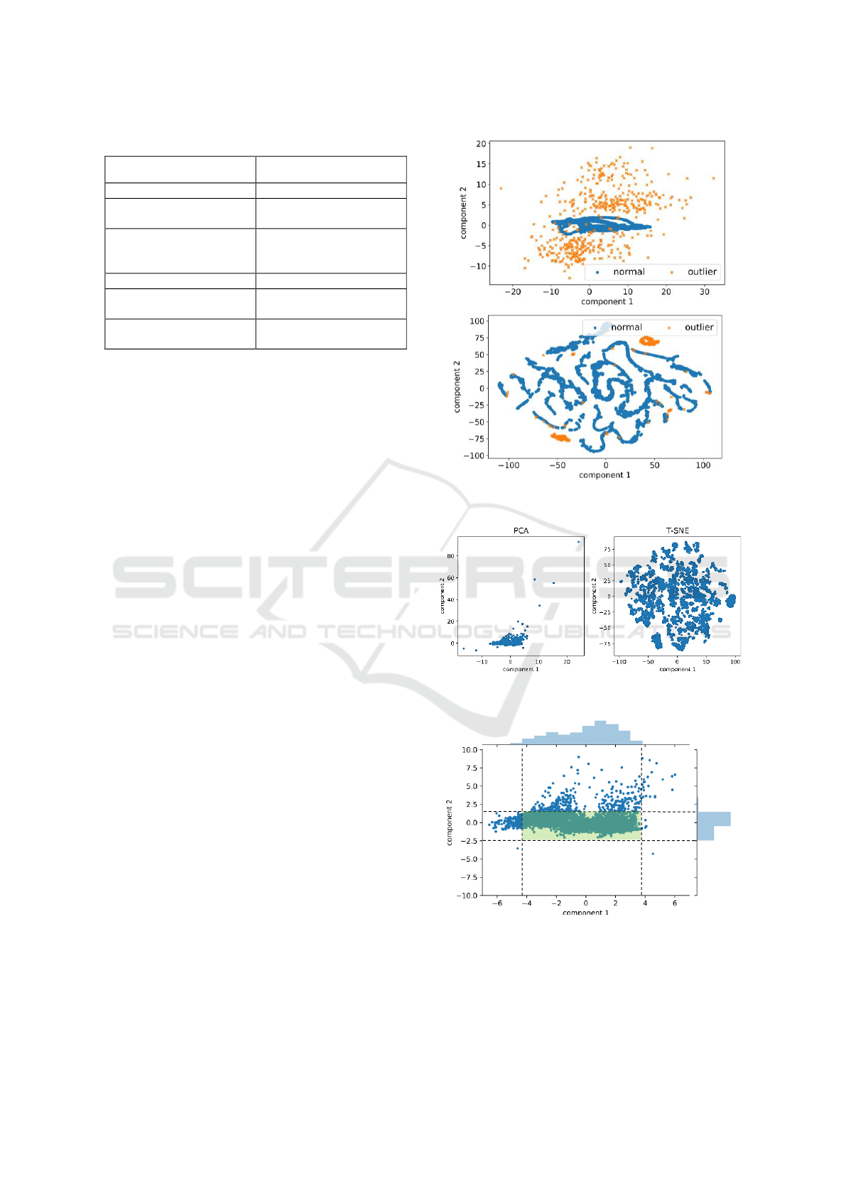
Table 2: Sensor on sensor node.
Sensor model
Variable
SHARP GP2Y1010AU0F
PM
SGX
MICS2614
O3
SGX
MICS6814
NO2, CO,CO2, O3, CH4,
NH3, H2, CH3H8 and
C4H10
CLE-0421-400
SO2
Sparkfun
SEN-12642
Acoustic pressure
DHT22
Temperature and
Humidity
PCA and T-SNE will be used to evaluate the EOD
because they allow the visualization of the data and
the detected outliers. PCA (Tipping and Bishop,
1999) is a lineal dimension reduction technique that
computes the Eigen vectors of a high dimensional
space and keeps the most relevant vectors to generate
a new low dimensional data space. T-SNE (van der
Maaten and Hinton, 2008). is a non-lineal dimension
reduction method that is able to maintain the original
distances between records. T-SNE will be crucial for
checking the kind of outlier detected. The global
outliers will usually share a cluster on the T-SNE
space while the local outliers will correspond to
isolated points on the reduced space.
Using these two techniques, we will be able to
reduce the dimensionality up to a 2D space where we
will visualize the new distribution and consider the
outliers as the records with higher distance to the
centre of mass of the data, in the case of PCA, and as
abnormal clusters, for the T-SNE.
In order to compare the labelled Intel dataset
results and the Growsmarter real use case, the PCA
and the T-SNE are also applied to the Intel data. Intel
data is already a 2 dimensional space, since only
temperature and humidity are considered. Hence, the
resulting dimensionality will be 2D again. In Figure
12 the transformations are applied to the Intel test data
with synthetic outliers. In the PCA, outliers are far
from the centre of mass and are located on
depopulated areas. T-SNE manage to group the
majority of outliers in two different clusters and the
reminder outlier records corresponds to isolated
points. These graphics give a better understanding of
what the outliers should look using these techniques.
Figure 12: PCA (top) and T-SNE (down) on Intel Test Data.
Figure 13: PCA (left) and TSNE (right) on original data:
Figure 14: Zoom in PCA and data density.
Similarly in Figure 13, the resulting 2D space for
the Growsmarter data is shown. In order to give a
clear visualization on where we expect to find the
outliers, a zoom in is performed in Figure 14. In this
Ensembled Outlier Detection using Multi-Variable Correlation in WSN through Unsupervised Learning Techniques
45
way we provide a green highlighted rectangle
containing the higher density areas on the data.
Taking the original 16-dimensionality data space,
we can train our EOD using all the data. As we do not
have any kind of label, a common issue on real data,
there are no reasons to split on train and test set. An
important parameter to take into account is the
contamination ratio. Depending on how we “relay”
on our sensor data or depending on how many
abnormal values we want to detect, we have to adjust
the contamination. The shown experiment is carried
out with a contamination of 4% which has been
empirically shown to give the better results.
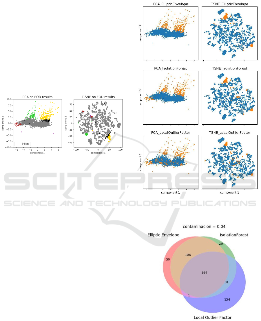
Figure 15: PCA and T-SNE with detected outliers
represented in colours according to its clustering in the T-
SNE.
The detected outliers are shown in Figure 15 using
different colours. All coloured points are detected
outliers using the EOD while the grey points are the
normal data. Then, we assign one colour to every
outlier cluster created by the T-SNE. Hence, we are
able to locate these clusters also in the PCA. It is clear
how the low density clusters and isolated points are
detected as outliers on PCA. Also the outliers on T-
SNE are grouped on clusters or are isolated records
on the space.
Although we are not able to have accurate metrics
due to the lack of labels, the EOD managed to
detected the low density areas of a 16 variable space
and detect the abnormal points isolated from the
others with a full unsupervised approach.
Moreover in Figure 16, we can see how the three
algorithms contributed to the final EOD decision.
Note that in this case, EOD detects outliers in the left
part of the PCA which EE cannot detect.
In Figure 17 we can see the Venn diagram of the
Growsmarter scenario. In this case, a total of 528
outliers are detected by at least one of the algorithms
with 334 of them being outliers according to the
EOD, which is the 63%.
Figure 16: PCA and T-SNE for the three algorithms:
Elliptic Envelope (top), Isolation Forest (middle) and Local
Outlier Factor (down) in the Growsmarter case.
Figure 17: Venn diagram of the Growsmarter case. All
outliers detected by at least two of the algorithms are
considered outliers by the EOD.
IoTBDS 2019 - 4th International Conference on Internet of Things, Big Data and Security
46

4.2 MUV
This work has also been considered as the main
technology for a proof-of-concept in the project
Mobility Urban Values (MUV) (MUV project, 2019),
where different monitoring stations are installed in 6
different European cities. These stations monitor not
only weather and pollution aspects but also include
noise and traffic sensing (including cars, bicycles and
pedestrians).
For weather and pollution the requirements and
the environment will be very similar to the one
presented in GrowSmarter. The main differences are
the static location of the stations, some slight changes
in the sensors requirements and the implementation in
6 cities which should be running the service
continuously.
However, the new sources of data (noise and
traffic), imply a high challenge for EOD for three
reasons. Firstly, these are new sources which are
highly correlated but that have a completely different
nature than the ones analysed in Growsmarter.
Secondly, the amount of data generated will be much
higher, since these sensors have a real-time sampling
rate. Finally, the noise sensor includes continuous
signal processing.
5 CONCLUSIONS
In this paper we have presented a construction of an
Ensemble Outlier Detector based on a majority voting
system using three different unsupervised learning
techniques, namely elliptic envelope (EE), isolation
forest (IF) and local outlier factor (LOF) based on
multi-variable correlation.
These three algorithms are evaluated using the
Intel Berkeley dataset, focusing only in the
temperature and humidity variables. The results of the
analysis using this dataset with synthetically added
outliers is extensively discussed. Then, we have
tested the system in a real case scenario as part of the
project Growsmarter, using bikes with sensors that
move around the city of Barcelona. The results are
shown graphically because of the difficulty to obtain
appropriate labelled datasets to perform a more
accurate analysis. Using spectral-decomposition
techniques, we are able to compare the results of the
EOD in the real scenario with the results obtained in
the Lab experiment. Our analysis concludes that the
behaviour is very similar and we can expect similar
results in terms of accuracy, detection and false alarm
rates in the real scenario with the ones that we have
obtained in the Lab case.
The overall result indicates that, for correlated
variables, the analysis performed using unsupervised
techniques is highly accurate. Furthermore, it permits
the use of Big Data approaches like Map Reduce,
since we do not focus on the temporal correlation of
the variables, hence we can analyse the samples
independently and without any order. This is a major
advance towards outlier detection in Big Data
systems.
The main stopper to an appropriate comparison of
different outlier detection techniques based on
different correlations in a real scenario is the need to
obtain real labelled datasets. A possibility is to install
a monitoring device close to a highly-accurate
measuring station and use the results to label the
device’s samples. However, if we talk about Smart-
Cities, measuring stations are usually installed in the
roofs of high buildings precisely to avoid sensor noise
produced close to the street. The resulting dataset can
be used to calibrate the sensors but is not useful to
evaluate the results of an outlier detection system
when the monitoring device is placed in the street in
its usual day-to-day scenario.
Another discovered advance is the resilience of
the EOD to different scenarios. While in simple
scenarios like the Intel Berkley dataset, Local Outlier
Factor and specially, Isolation Forest, give bad and
very divergent results, the EOD is able to stay close
to the good results given by EE. In complex scenarios
like the 16-dimensionality where the three algorithms
converge more, LOF and IF give better results and the
EOD is adapting even better and providing very good
overall detection.
A major advance in outlier detection in Big Data
systems would be the creation of a real and large
labelled dataset with multiple correlated and non-
correlated variables. This dataset would set a baseline
where different approaches can be compared not only
in terms of accuracy, detection rate and false alarm
rate, but also in terms of performance and adaption to
big data scenarios.
A complete comparison of different algorithms
and different correlations could help to create much
better systems that can effectively work in real IoT
deployments.
ACKNOWLEDGEMENTS
Authors would like to thank the Growsmarter and
MUV projects, which have received funding from the
European Union’s Horizon 2020 research and
innovation programme under grant agreements no.
646456 and no. 723521 respectively.
Ensembled Outlier Detection using Multi-Variable Correlation in WSN through Unsupervised Learning Techniques
47

REFERENCES
Barakkath Nisha U, Uma Maheswari N.; Venkatesh R., and
Yasir Abdullah R, 2014. “Robust estimation of
incorrect data using relative correlation clustering
technique in wireless sensor networks”. Proceedings of
the International Conference on Communication and
Network Technologies (ICCNT). Sivakasi, India.
Breunig M. M., Kriegel H. P., Ng R. T., and Sander, J.,
2000. “LOF: identifying density-based local outliers”.
Proceedings of the ACM SIGMOD 2000 Int. Conf. On
Management of Data. Dallas, Texas, USA.
Dean J., and Ghemawat S., 2008. “MapReduce: simplified
data processing on large clusters”. In Communications
of the ACM, volume 51, issue 1, pp 107-113.
Elnahawy E. and Natch B., 2003. “Cleaning and querying
noisy sensors”. Proceedings of the 2
nd
ACM Interna-
tional conference on Wireless sensor networks and
applications (WSNA). San Diego, CA, USA. pp 78-87.
Ghorbel O., Ayedi W., Snoussi H. and Abid M., 2015. “Fast
and efficient outlier detection method in Wireless
Sensor Networks”. IEEE Sensors Journal, Vol 15, No
6, pp. 3403-3411
Growsmarter project web site. Available at:
http://www.grow-smarter.eu/ Last accessed 14/02/2019
Intel Berkeley Research Lab. Available at:
http://db.csail.mit.edu/labdata/labdata.html. Last
Jones E., Oliphant T. and Peterson P., 2018. “SciPy: Open
Source Scientific Tools for Python”. Online Code
Repos. Available at: http://www.scipy.org/
Liu, F. T., Ting, K. M. and Zhou, Z., 2008. “Isolation
forest”. Proceedings of the Eighth IEEE International
Conference on Data Mining. Pisa, Italy. pp 413-422.
MUV: Mobility Urban Values project web site. Available
at:https://www.muv2020.eu/. Last accessed 14/02/2019
Pena F.L., Eiroa A.B., Duro R.J., 2003. “A virtual
instrument for automatic anemometer calibration with
ANN based supervision”. IEEE Transactions on
Instrumentation and Measurement. Vol 52, Issue 3, pp
654-661.
Rousseeuw P.J. and Van Driessen K., 1999. “A fast
algorithm for the minimum covariance determinant
estimator”. Technometrics. Volume 41, issue 3, pp 212-
223.
Shikha Shukla, D., Chandra Pandew, A., Kulhari, A., 2014.
“Outlier Detection: A Survey on Techniques of WSNs
Involving Event and Error Based outliers”. Proceedings
of the International Conference of Innovative
Applications of Computational Intelligence on Power
Energy and Controls with their Impact on Humanity
(CIPECH14). Ghaziabad, India.
Shvachko K., Kuang H., Radia S., and Chansler R.. 2010.
“The Hadoop Distributed File System”. Proceedings of
the IEEE 26th Symposium on Mass Storage Systems
and Technologies (MSST). Incline Village, Nevada,
USA.
Spinelle L., Gerboles M., Gabriella Villani M. Aleixandre
M. and Bonavitacola F., 2015. “Field calibration of a
cluster of low-cost available sensors for air quality
monitoring. Part A: Ozone and nitrogen dioxide”.
Proceedings of the IEEE International Workshop on
Virtual and Intelligent Measurement (VIMS2001).
Budapest, Hungary.
Stanway A., 2013. “Etsy Skyline”. Online Code Repos.
Available at: https://github.com/etsy/skyline
Tipping M. E., and Bishop C. M., 1999. “Probabilistic
principal component analysis”. Journal of the Royal
Statistical Society, Series B, 61, Part 3, pp. 611-622.
van der Maaten, L and Hinton G., 2008. “Visualizing Data
using t-SNE”. Journal of Machine Learning Research
9, pp. 2579-2605.
Yang Z., Meratnia N., and Havinga P., 2008. “An online
outlier detection technique for wireless sensor networks
using unsupervised quarter-sphere support vector
machine”. Proceedings of the International Conference
on Intelligent Sensors, Sensor Networks and
Information Processing (ISSNIP 2008). Sydney,
Australia. pp. 151 –156.
Zaharia M., Xin R.S., Wendell P., Das T., Armbrust M.,
Dave A., Meng X., Rosen J., Venkataraman S.,
Franklin M.J., Ghodsi A., Gonzalez J., Shenker S, and
Stoica I.. 2016. “Apache Spark: a unified engine for big
data processing”. Communications of the ACM. volume
59, issue 11, pp. 56-65.
Zheng W., Yang L., and Wu M, 2018. “An Improved
Distributed PCA-Based Outlier Detection in Wireless
Sensor Network”. Proceedings of the Cloud
Computing and Security (ICCCS2018). Haikou, China.
IoTBDS 2019 - 4th International Conference on Internet of Things, Big Data and Security
48
