The ε-approximation of the Label Correcting Modiﬁcation of the

Dijkstra’s Algorithm

Franti

sek Kolovsk

, Jan Je

zek

and Ivana Kolingerov

Depatment of Geomatics, University of West Bohemia, Univerzitn

ı 2732/8, Plze

n, Czech Republic

Department of Computer Science, University of West Bohemia, Univerzitn

ı 2732/8, Plze

n, Czech Republic

Keywords:

Time-dependent Shortest Path Problem, Approximation, Travel Time Function, Road Network.

Abstract:

This paper is focused on searching the shortest paths for all departure times (proﬁle search). This problem

is called a time-dependent shortest path problem (TDSP) and is important for optimization in transportation.

Particularly this paper deals with the

-approximation of TDSP. The proposed algorithm is based on a label

correcting modiﬁcation of Dijkstra’s algorithm (LCA). The main idea of the algorithm is to simplify the arrival

function after every relaxation step so that the maximum relative error is maintained. When the maximum

relative error is 0.001, the proposed solution saves more than 95% of breakpoints and 80% time compared to

the exact version of LCA. A more efﬁcient precomputation step for another time-dependent routing algorithms

can be built using the developed algorithm.

1 INTRODUCTION

Computing the arrival function from a source node

to all other nodes is important for a lot of transporta-

tion applications. More formally, given a directed

graph

G = (V, E)

, a source node

s ∈ V

, we want to

know the travel time between the source node

and all

other nodes for every departure time (in some literature

called a travel time proﬁle). This problem is gener-

ally called the time-dependent shortest path problem

(TDSP). The main principle is that the arrival time

at the node

is used as the argument of the arrival time

function

corresponding with the edge that origins at

The common approach is to use a piecewise linear

function as a realization of the arrival function. Let us

have two consecutive edges (e.g, the edges

(s, u)

and

(u, d)

in Figure 1a) then the arrival time at the node

the value of the arrival function

in the arrival time

)

at the node

, where

is the departure time at

the node

. In the exact case, the combination

( f

(t))

of two piecewise linear functions

with

| f

linear pieces is also a piecewise linear function with

up to

| f

| + | f

linear pieces (Foschini et al., 2014). It

means that the arrival function at the end of the path

with

edges can have up to

∑

i=1

| f

linear pieces. For

example, the path across the Pilsen city has around

100 edges. If every arrival function on the path has 24

linear pieces, the resulting arrival function has 2400

liner pieces. It can be seen that the computational time

and memory requirements strongly increases with the

length of the paths.

The problem with an increase in the number of lin-

ear pieces can be solved using the

-approximation of

the resulting arrival function. This approach reduces

the number of linear pieces and thus reduces mem-

ory requirements as well as computation time. Our

proposed algorithm is based on the so-called label cor-

recting modiﬁcation of Dijkstra’s algorithm (Orda and

Rom, 1990). The main idea is to perform a simpliﬁ-

cation of the arrival functions during the computation

with a suitable maximum absolute error such that the

relative error ε is maintained.

2 DEFINITIONS AND

PRELIMINARIES

2.1 Road Network

Let

G = (V, E)

be a directed graph that represents a

road network, where

is a set of nodes and

is a set

of edges. Each edge

(u, v) ∈ E

has an arrival function

(AF)

f : R → R

≥0

that for the given departure time

returns the arrival time at

. Alternatively, we

can deﬁne a travel time function (TTF) that returns the

time needed to cross the edge. A relationship between

Kolovský, F., Ježek, J. and Kolingerová, I.

The e-approximation of the Label Correcting Modiﬁcation of the Dijkstra’s Algorithm.

DOI: 10.5220/0007658200260032

In Proceedings of the 5th International Conference on Geographical Information Systems Theory, Applications and Management (GISTAM 2019), pages 26-32

ISBN: 978-989-758-371-1

the TTF

and the corresponding AF

is deﬁned as

g(t) = f (t) − t.

It is assumed that every AF

fulﬁll the FIFO prop-

erty:

∀t

< t

: f (t

) ≤ f (t

)

and the departure time

must be smaller then the arrival time

(the travel time

must be positive). AFs are implemented as piecewise

linear functions.

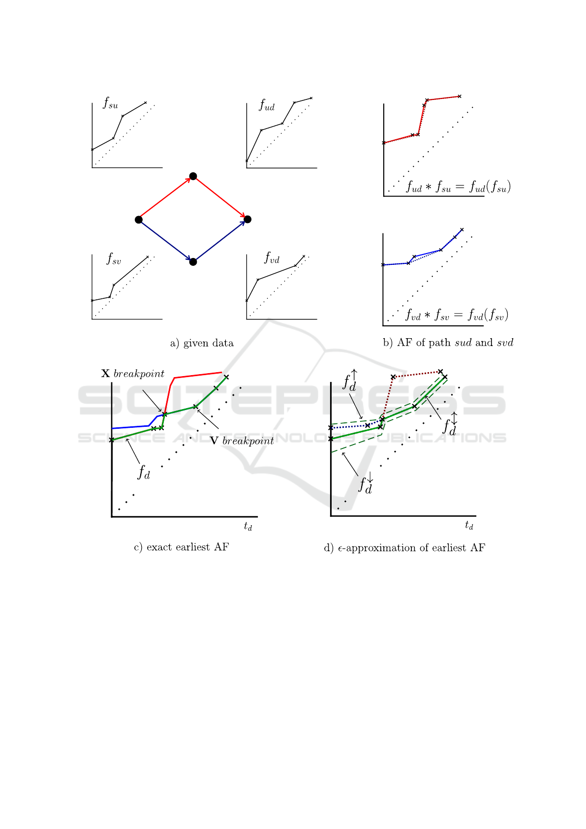
In Figure 1a you can see AFs (

and

) for every edge in a small example graph

with four nodes

V = {s, u, v, d}

and four edges

E =

{(s, u), (s, v), (u, d), (v, d)}.

The points of AFs are called breakpoints. The

number of breakpoints of AF

can be written as

| f |

The following operation must be deﬁned for two AFs:

•

There are two consecutive edges

(s, u)

and

(u, d)

with AFs

. The operation combination

∗ f

: t 7→ f

( f

(t))

represents AF from

. In Figure 1b there are AFs as results of the com-

bination along the paths

(s, u, d)

(solid red line)

and (s, v, d) (solid blue line).

•

There are two parallel paths

from

with AFs

. The operation minimum

min( f

, f

) : t 7→ min{ f

, f

}

represents the ear-

liest AF from

. In Figure 1a

= (s, u,d)

and

= (s, v, d)

. In Figure 1c you can see this earliest

AF as a result of the operation minimum (green

line).

2.2 Problem Deﬁnition

More precisely, TDSP can be deﬁned as minimizing

the travel time over the set

s,d

of all paths in

from

the source node s to the destination node d:

= min{ f

(t)|p ∈ P

s,d

} (1)

where

is the function of the earliest arrival time

(minimal AF) from

and

is AF of the path

p ∈ P

s,d

This paper deals with one-to-all problem. The

input data are the graph

, AF

for every edge

(u, v) ∈ G

and the source node

. The output is the

set

of the earliest AFs from the source node

to all

other nodes u: F = {f

|u ∈ V \ {s}}.

2.3 Approximation

In this paper the

-approximation of AF

is under-

stood as the

-approximation of TTF

f (t) − εg(t) ≤

(t) ≤ f (t) + εg(t)

. So the

-approximation of the

set F is F

= { f

|u ∈ V \ {s}}.

Let us present some useful theorems about the ap-

proximation that were derived for a use in the proposed

algorithm.

Theorem 1.

Let

be an

-approximation of TTF

Then it holds that

↓

1 + ε

≤ g ≤

1 − ε

= g

↑

Proof.

If the function

is substituted by its extreme

values

(1 − ε)g

(1 + ε)g

, the expression is still valid.

Theorem 2.

Let

be an

-approximation of AF

and

= f

∗ f

. Let

α ∈ [0,

↓

]

be the maximum

slope of AF

approx( f , δ)

be a function that sim-

pliﬁes the AF

with the maximum absolute error

δ ≥ 0

. Then

= approx( f

, εg

↓

− αεg

↓

)

is the

approximation of AF f

Proof.

The maximum absolute error of

εg

and

the maximum absolute error of the operation

∗ f

αεg

. Then the result of the combination can be

simpliﬁed with the maximum absolute error:

δ = εg

− αεg

≥ εg

↓

− αεg

↓

Then δ must be ≥ 0

εg

↓

− αεg

↓

≥ 0

α ≥

↓

Theorem 2 can be also formulated in a local form

for a given departure time.

In Figure 1b there are dotted lines that represent

the approximation of AFs. In Figure 1d you can see

the

-approximation

of the earliest AF

from

(solid green line) and its upper bound

↑

and lower

bound f

↓

(green dashed lines).

2.4 Related Work

There are two groups of methods that compute an ap-

proximation of the AF. The ﬁrst methods use forward

and backward probes. The forward probe computes

the arrival time at the node

with the given departure

time at the node

. The backward probe solves the

inverse problem. The arrival time at

is given and we

want to know the departure time at

. These probes

can be computed using the well-known Dijkstra’s al-

gorithm (Dehne et al., 2012).

These methods recognize two types of breakpoints.

The

points represent points that are created as im-

ages of the breakpoints that lie on the edge arrival

The e-approximation of the Label Correcting Modiﬁcation of the Dijkstra’s Algorithm

Figure 1: Example of calculation of the arrival function from node s to d.

functions

{ f

|(u, v) ∈ E}

. The

points are created

as an intersection of two AF in the

minimum

operation.

It can be proved that the AF between two consecu-

tive

points is concave or a line segment (Foschini

et al., 2014) (see Example in Fig. 1c). The algo-

rithms described in (Foschini et al., 2014), (Omran

and Sack, 2014) use this concavity. First the V points

are computed using one backward probe and two for-

ward probes (more in (Dehne et al., 2012)) and then

the approximation of AF between the

points is de-

termined. The main problem of this approach is that

the computation of

points requires

∑

(u,v)∈E

| f

probes (Dehne et al., 2012).

The second group of methods uses a label correct-

ing modiﬁcation of the Dijkstra’s algorithm (LCA)

(Algorithm 1). The modiﬁcations of the Dijkstra’s

algorithm are:

• The node labels are AFs from s.

•

The key of the priority queue is the minimum of

AF (min f ).

•

The relaxation of the edge

(u, v)

is performed using

GISTAM 2019 - 5th International Conference on Geographical Information Systems Theory, Applications and Management

= min( f

, f

∗ f

)

LCA has time complexity

O(|V ||E|)

(Orda and

Rom, 1990), but a real road network is far from the

worst case. This technique is widely used, see e.g,

(Geisberger and Sanders, 2010) (Batz et al., 2013)

(Geisberger, 2010). First LCA is performed in the

exact form and after that the resulting arrival functions

are simpliﬁed and used for further computation (e.g,

some query algorithm). Some guarantees about the

error of AF are presented in (Geisberger and Sanders,

2010), but these guarantees give only a maximum

error dependent on the degree of approximation.

Algorithm 1: LCA in the exact form.

1 PQ = minimum priority queue where key is

min f

2 ∀u ∈ V : f

= ∞

3 g

= 0

4 PQ.put( f

)

5 while queue is not empty do

6 f

= PQ.get()

7 foreach v : (u, v) ∈ E do

8 f

= f

∗ f

// combination

9 if ∃t : f

(t) < f

(t) then // compare

10 f

= min( f

, f

) // min

11 PQ.put( f

)

In Algorithm 1 the initialization is performed in

the lines 1-4. All node labels (AFs) are set to inﬁnity

in the line 2. The travel time at

is set to zero (line

3) and the node label at

(

) is added to the priority

queue (PQ) (line 4). In the line 6 the algorithm takes

the node on the top of PQ and relaxes all edges that

lead from this node. The relaxation is represented by

the lines 8-11. The line 8 performs the combination

of the node label at

(

) and the edge AF (

). The

condition in the line 9 checks for update. Updates of

the label at the node

are performed in the line 10.

The line 11 puts the node v to the PQ.

The main task is to develop an algorithm which

solves TDSP with the given maximum relative error

and is effective for a real road network. It follows that

we focused on the ε-approximation of the LCA.

3 PROPOSED ALGORITHMS

This section describes two algorithms solving the

approximation of TDSP based on LCA (Algorithm

1).

3.1 ε-LCA Algorithm

The basic idea of the ﬁrst proposed algorithm (

-LCA)

is that the simpliﬁcation of AF is performed after ev-

ery edge relaxation (the operation combination). The

degree of the simpliﬁcation is directed by Theorem 2.

The

-LCA computes AF with the maximum rela-

tive error ε assuming that

∀(u, v) ∈ E : α

∈

↓

(2)

where

is the maximum slope of AF

. The slope

must be bounded because Theorem 2 is used in

the ε-LCA and the theorem needs this assumption.

The

-LCA differs from the exact LCA only in

the computation of

. The AF

in the line 8 in

Algorithm 1 is simpliﬁed with the maximum absolute

error

(according to Theorem 2). So the line 8 is

replaced by 2 lines

δ(t) = ε(( f

∗ f

)

↓

(t) −t) − α(t)εg

↓

(t)

= approx(( f

∗ f

), δ)

(3)

where

α(t)

is the maximum slope of

in the interval

[ f

↓

(t), f

↑

(t)]

. The simpliﬁcation was performed using

Douglas-Peucker algorithm or Imai and Iri algorithm

(Imai and Iri, 1986).

The main problem of

-LCA is that if the assump-

tion

(2)

is not complied,

δ < 0

and the algorithm can-

not ensure the given relative error

. This occurs when

the maximum slope

is too large. This issue is re-

solved using the second algorithm that is described in

the upcoming section.

3.2 ε-LCA-BS Algorithm

The second proposed algorithm (

-LCA-BS) is based

on backsearch. It has no limitations for the slope

The pseudo-code of the

-LCA-BS is in Algorithm

2. The basic idea is that if the algorithm ﬁnds an

edge

(u, v)

where

is too big in some departure time

interval

]

(

δ < 0

), it determines

]

again

with a higher accuracy (lines 11-15 of the Algorithm

2). The algorithm returns back to the point such that

the edge

(u, v)

can be reached from this point with

sufﬁcient precision using the exact LCA.

When the label at the node

(AF

) is updated

(the condition at the line 16 is fulﬁlled), the edge

(u, v)

is added to the predecessor list

pred(v)

of the node

(lines 17-20). The set of predecessors form a graph

R = (V

, E

)

(red color in Fig. 2). We assume that the

graph

is acyclic. In general, the graph

may not be

acyclic, but in real case it is very unlikely.

The e-approximation of the Label Correcting Modiﬁcation of the Dijkstra’s Algorithm

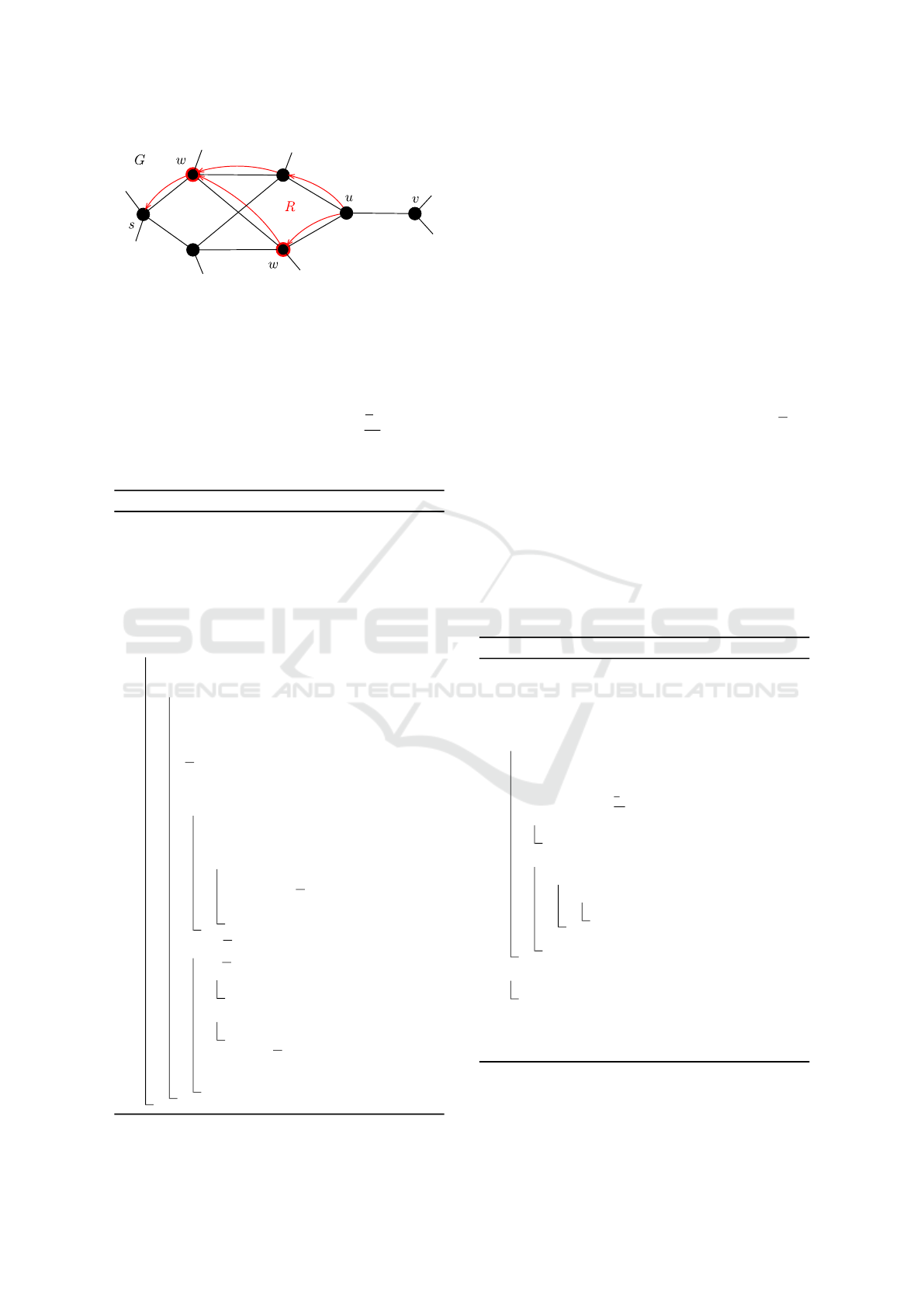
Figure 2: Example of backsearch procedure.

We want to ﬁnd nodes

such that if the exact

LCA is performed from these nodes

, the AF

-approximation. The nodes

have to satisfy the

following inequalities in the interval [t

max

(

∏

e∈p

|p ∈ P

)

≤ min

↓

(4)

Algorithm 2: ε-LCA-BS.

1 PQ = minimum priority queue where key is

min f

2 ∀u ∈ V : f

= ∞

3 g

= 0

4 PQ.put( f

)

5 pred(s) = null

6 while queue is not empty do

7 f

= PQ.get()

8 foreach v : (u, v) ∈ E do

9 δ(t) =

ε(( f

∗ f

)

↓

(t) −t) − α(t)εg

↓

(t)

// according equation 3

10 f

= approx( f

∗ f

, δ

)

// δ

(t) = max(δ(t), 0)

11 if ∃t : δ(t) < 0 then

12 ﬁnd all intervals [t

] where δ is

negative

13 foreach [t

] do

14 h = backSearch((u, v),[t

])

15 substitute f

by h in interval

]

16 if ∃t : f

(t) < f

(t) then

17 if f

< f

then

18 pred(v) = (u, v)

19 else

20 pred(v).add((u, v))

21 f

= min( f

, f

)

22 PQ.put( f

)

where

is the set of all paths from

in the

graph

(the paths must contain the edge

(u, v)

) and

represents the maximum slope of AF

corresponding

with the edge

. The set

is the set of all nodes

that meet the condition

(4)

and there is a path

p ∈ P

that does not contain any other node from the set

(W is the smallest possible).

These nodes

can be found using a topological

ordering of

(Algorithm 3). The node labels

correspond to the left side of the inequalities

(4)

. So

the algorithm ﬁnds maximal paths in

. First the labels

are set to negative inﬁnity (the line 2) and the label

is set to

(the line 3). The lines 4-5 ensure a

topological ordering. If the condition

(4)

in the line

6 is fulﬁlled,

is added to the

. The lines 9-12

ensure updating of the node labels. The part of

the interval

]

is substituted by a more accurate

result of the exact LCA with the initial priority queue

PQ that is created by adding all

∈ { f

|w ∈ W}

(the

lines 13-16).

In Figure 2 there is an example of backsearch. The

black color represents the original graph

and the red

color represents the acyclic graph

. The edge

(u, v)

violates the condition 2. Then the algorithm starts

backSearch procedure and ﬁnds the set

(red nodes)

using the graph R.

Algorithm 3: backSearch.

1 W = {} // set of all w

2 ∀b ∈ V

: α

= −∞

3 α

= α

4 while ∃b : b ∈ V

\W ∧ deg

−

(b) = 0 do

// topological ordering

5 b = some node that meets the conditions

above

6 if α

≤ min



↓



then

7 W = W ∪{b}

8 else

9 foreach a : (b,a) ∈ R do

10 if α

> α

then

11 α

= α

12 V

= V

\ {b}

13 foreach w ∈ W do

14 PQ.put( f

)

15 run LCA on G with initial priority queue PQ

on interval [t

] // algorithm 1

16 return f

When the graph

is not acyclic, it is necessary to

modify the algorithm for searching the set W .

GISTAM 2019 - 5th International Conference on Geographical Information Systems Theory, Applications and Management

If the condition

(2)

is fulﬁlled, the

-LCA-BS is

reduced to

-LCA, because the algorithm then does

not perform any backSearch procedure.

4 EXPERIMENTS

The real road network with real speed proﬁles that

were computed from GPS tracks was used for testing.

This data represent part of Paris in France (Figure 3).

Figure 3: Route network for testing.

The algorithms were implemented using Scala pro-

gramming language (OpenJDK 1.8, Debian 10). The

testing was performed on a computer with Intel(R)

Core(TM) i5-8250U CPU @ 1.60GHz and with 16

GB RAM. One thread was used only.

Table 1: Graph properties (#edges - number of edges,

| f

number of linear pieces of AF for each edge).

dataset #edges | f

G1 10 798 24

G2 33 354 24

G3 107 476 24

G4 160 092 24

Table 2: Absolute values of measured parameters for

ε =

0.001.

Imai and Iri Douglas Peucker

time [s] # bps time [s] # bps

G1 0.5 608 k 1.0 940 k

G2 1.9 2 087 k 3.9 3 136 k

G3 6.4 5 734 k 13.3 8 606 k

G4 9.6 7 876 k 20.2 11 892 k

The

-LCA-BS was tested only because

-LCA

is a special case of

-LCA-BS only. The maximum

allowed relative error

was set to

−1

, 10

−2

, 10

−3

and 10

−4

Four graphs (G1, G2, G3 and G4) were created

to show the performance of the developed algorithms.

Every edge in the graphs has AF with 24 linear pieces.

Table 3: Results of testing

-LCA-BS (

- the relative time

related to the exact version of LCA,

bps

- the relative number

of breakpoints, ε - the maximum allowed relative error).

Imai and Iri Douglas Peucker

ε t

[%] bps [%] t

[%] bps [%]

G1 10

−1

3.9 0.1 7.0 0.2

−2

6.0 0.8 6.4 0.9

−3

16.4 3.1 32.3 4.9

−4

45.2 10.6 104.7 15.3

G2 10

−1

1.7 0.1 1.5 0.1

−2

4.1 0.6 4.7 0.7

−3

14.0 3.0 27.1 4.6

−4

42.0 10.6 97.3 15.4

G3 10

−1

1.5 0.1 1.5 0.1

−2

3.5 0.5 3.3 0.5

−3

11.1 2.5 21.4 3.8

−4

37.5 9.4 86.5 14.2

G4 10

−1

1.4 0.1 1.0 0.1

−2

3.3 0.5 3.3 0.5

−3

10.5 2.4 20.3 3.6

−4

35.3 8.8 82.8 13.7

Every graph represents different classes of roads. In

Table 1 there are numbers of edges for each graph.

In Table 3 there are performance results of

-LCA-

BS: the relative time

and the relative number of

breakpoints

bps

related to the exact version of LCA.

The same results you can see in Figure 4.

The results in Table 3 show that the maximum rel-

ative error

−4

brings only a small improvement, but

this accuracy is too big for a real use. The maximum

relative error from

−2

−3

seems to be a good

compromise between accuracy and performance.

In Table 2 there are absolute values of measured

parameters for the maximal relative error

−3

. The

column

bps

represents the number of breakpoints in

the resulting AFs. In all cases the graphs (G1-G4) do

not violate the condition

(2)

, thus the

-LCA-BS was

reduced to ε-LCA.

The results show that the breakpoints savings are

signiﬁcant. It means that the

-LCA-BS saves a lot of

memory. Let us assume a path that takes 1 hour, then

the relative error 0.1 % implicates the absolute error

3.6 s. In this case the epsilon approximation saves

more than 95% of memory and 80% of time. In case

that

is too small then the algorithm can run slower

than the exact version, because the simpliﬁcation takes

too much time.

The main disadvantage of the

-LCA-BS is that it

is sensitive to values of the maximum slope of AFs. If

AFs have too big slope then the algorithm performs

too many calls of backSearch procedure and thereby

makes the computation too slow. In practice, the func-

The e-approximation of the Label Correcting Modiﬁcation of the Dijkstra’s Algorithm

Figure 4: The relative number of breakpoints and the relative time related to exact LCA (II - Imai and Iri, DP - Douglas

Peucker).

tions usually have small slopes. When it is certain

that input data do not violate the condition

(2)

, the

algorithm is more suitable.

5 CONCLUSION

Two algorithms for

-approximation of TDSP were

presented. The algorithms signiﬁcantly reduce the

memory use. When the maximum relative error is a

sufﬁciently large value (in our case

−3

), the algo-

rithms save the computational time too. From this

point of view, the algorithms are suitable for precom-

puting the TTFs for the next use (e.g., time-dependent

distance oracles, time-dependent contraction hierar-

chies).

In a real road network the maximum slopes of

AFs are not too big (Strasser, 2017). So the main

disadvantage (too many calls of back search procedure)

is not a too big problem. In one-to-one problem case

the developed algorithms can be combined with other

speed-up techniques that reduce the graph (e.g., time-

dependent-sampling (Strasser, 2017)).

In the future work it would be useful to use some

heuristics for decision whether it is necessary to per-

form backSearch. The goal is to remove the cases

when the difﬁcult-to-calculated AF (using backSearch)

is fully replaced by another AF from another node.

ACKNOWLEDGEMENTS

This work has been supported by the Project SGS-

2019-015 (”Vyu

zit

ı matematiky a informatiky v geo-

matice IV”) and by Ministry of Education, Youth and

Sports of the Czech Republic, the project PUNTIS

(LO1506) under the program NPU I

REFERENCES

Batz, G. V., Geisberger, R., Sanders, P., and Vetter, C. (2013).

Minimum time-dependent travel times with contraction

hierarchies. Journal of Experimental Algorithmics,

18:1.1–1.43.

Dehne, F., Omran, M. T., and Sack, J.-R. (2012). Shortest

Paths in Time-Dependent FIFO Networks. Algorith-

mica, 62(1-2):416–435.

Foschini, L., Hershberger, J., and Suri, S. (2014). On the

Complexity of Time-Dependent Shortest Paths. Algo-

rithmica, 68(4):1075–1097.

Geisberger, R. (2010). Engineering Time-dependent One-

To-All Computation. arXiv:1010.0809 [cs]. arXiv:

1010.0809.

Geisberger, R. and Sanders, P. (2010). Engineering time-

dependent many-to-many shortest paths computation.

In OASIcs-OpenAccess Series in Informatics, vol-

ume 14. Schloss Dagstuhl-Leibniz-Zentrum fuer In-

formatik.

Imai, H. and Iri, M. (1986). An optimal algorithm for ap-

proximating a piecewise linear function. Journal of

information processing, 9(3):159–162.

Omran, M. and Sack, J.-R. (2014). Improved approximation

for time-dependent shortest paths. In International

Computing and Combinatorics Conference, pages 453–

464. Springer.

Orda, A. and Rom, R. (1990). Shortest-path and minimum-

delay algorithms in networks with time-dependent

edge-length. Journal of the ACM (JACM), 37(3):607–

625.

Strasser, B. (2017). Dynamic Time-Dependent Routing

in Road Networks Through Sampling. In OASIcs-

OpenAccess Series in Informatics, volume 59. Schloss

Dagstuhl-Leibniz-Zentrum fuer Informatik.

GISTAM 2019 - 5th International Conference on Geographical Information Systems Theory, Applications and Management