Continuously Improving Model of Road User Movement Patterns using
Recurrent Neural Networks at Intersections with Connected Sensors
Julian Bock
1
, Philipp Nolte
2
and Lutz Eckstein
1
1
Institute for Automotive Engineering (ika), RWTH Aachen University, Steinbachstr. 7, Aachen, Germany
2
RWTH Aachen University, Aachen, Germany
Keywords:
Prediction, Vulnerable Road Users, Pedestrian, Deep Learning, Automated Driving, Intersections.
Abstract:
Intersections with connected infrastructure and vehicle sensors allow observing vulnerable road users (VRU)
longer and with less occlusion than from a moving vehicle. Furthermore, the connected sensors are providing
continuous measurements of VRUs at the intersection. Thus, we propose a data-driven prediction model,
which benefits of the continuous, local measurements. While most approaches in literature use the most
probable path to predict road users, it does not represent the uncertainty in prediction and multiple maneuver
options. We propose the use of Recurrent Neural Networks fed with measured trajectories and a variety
of contextual information to output the prediction in a local occupancy grid map in polar coordinates. By
using polar coordinates, a reliable movement model is learned as base model being insensitive against blind
spots in the data. The model is further improved by considering input features containing information about
the static and dynamic environment as well as local movement statistics. The model successfully predicts
multiple movement options represented in a polar grid map. Besides, the model can continuously improve the
prediction accuracy without re-training by updating local movement statistics. Finally, the trained model is
providing reliable predictions if applied on a different intersection without data from this intersection.
1 INTRODUCTION
The 2015 status report on road safety by the World
Health Organization states that 1.25 million road traf-
fic deaths occur every year (WHO, 2016b). 275.000
of those 1.25 million or 22 % are pedestrians and an
additional 4 % are bicyclists. This is mainly due to
the fact, that those two groups belong to the class of
non-motorized road users, which are the most vulner-
able class, the Vulnerable Road Users (VRUs). The
WHO states that it is an important goal to make traf-
fic participation for VRUs safer. (WHO, 2016a).
In general, pedestrians are advised to cross a street
only at designated crosswalks or intersections with
traffic lights. However, especially at intersections
with multiple driving lanes or at unsignalized inter-
sections, pedestrians must keep attention on the traf-
fic. Using a mobile phone while crossing a street
can lead to a severe lack of attention and fatal acci-
dents (Hatfield and Murphy, 2007). Automated and
assisted driving should help to prevent accidents be-
tween VRUs and vehicles. However, especially in
urban scenarios, where scenes are cluttered by ob-
stacles, trees and other cars, the onboard sensors are
limited. In order to still be able to recognize pedestri-
ans with high precision, cooperative perception sys-
tems could be used (Kim et al., 2013). Those systems
use the fusion of sensor data from different sources
to model a more precise surrounding of the car than
by using the on-board sensors alone. For that, the car
communicates not only with other cars but also with
the infrastructure via Vehicle-to-Everything (V2X)
communication (Rauch et al., 2012).
Sensors integrated into the infrastructure can pro-
vide an elevated view on crowded scenes and of-
fer very precise sensor data about all traffic partic-
ipants. This approach was investigated in research
by e.g. the I2EASE project. Within the project, in-
formation from infrastructure sensors, vehicle sen-
sors and VRU localization devices is sent to a cen-
tral intersection computer to generate a fusion of all
the incoming data, which then can be used for fur-
ther applications such as the prediction of road user
movement. (Bock et al., 2017). Another project in-
specting the use of infrastructure mounted sensors
and X2X-communication station is the research in-
tersection built by DLR in Braunschweig, Germany
(Schnieder et al., 2016). They installed four multi-
Bock, J., Nolte, P. and Eckstein, L.
Continuously Improving Model of Road User Movement Patterns using Recurrent Neural Networks at Intersections with Connected Sensors.
DOI: 10.5220/0007675603190326
In Proceedings of the 5th International Conference on Vehicle Technology and Intelligent Transport Systems (VEHITS 2019), pages 319-326
ISBN: 978-989-758-374-2
Copyright
c
 2019 by SCITEPRESS – Science and Technology Publications, Lda. All rights reserved
319

sensor systems to measure road users at this inter-
section. Such data could be used in the context of
cooperative driver assistance systems or complete au-
tonomous driving features.
Sensors integrated into the infrastructure can not
only help to prevent accidents but also to improve traf-
fic flow, especially on crowded hot-spots like intersec-
tions (van Arem et al., 2006). Automated or assisted
driving functions can prevent critical situations with
pedestrians before they actually happen by predicting
the movement of pedestrians. For this, data-driven
machine learning approaches can be used.
2 RELATED WORK
In 2015, Goldhammer et al. (Goldhammer et al.,
2014) developed a Neural Network (NN) to predict
a pedestrians trajectory for the next 2.5 seconds. The
approach of using a NN was used to compare its ca-
pabilities in contrast to the commonly used Kalman-
filter method and approaches using only a NN without
polynomial input. The data for training the NN was
acquired by installing a camera at an intersection and
filming uninstructed pedestrians in a natural environ-
ment and the used network was a multi-layer percep-
tron. The result was a significantly better prediction
performance than with the Kalman-filter and also bet-
ter performance than predicting the trajectory without
the polynomial input .
Another approach of predicting pedestrians trajec-
tories with NNs was presented in 2017 by Pfeiffer et
al. (Pfeiffer et al., 2017). They integrated the sur-
roundings of the pedestrians into the prediction to in-
clude static obstacles influencing the path. Another
difference is, that they used a grid map to store not
only information about static surroundings but also
information about other pedestrians, which inundate
the observed one. Used data were a combination of
simulated data and the ETH dataset (Pellegrini et al.,
2009). The prediction task was interpreted as a se-
quence modeling task, therefore a Long Short-Term
Memory (LSTM) network was used. The complete
network consists of a joint LSTM, which takes three
inputs: The first input is the current velocity of the
observed pedestrian, the second is a two-dimensional
occupancy grid, which holds information about static
obstacles in the area. The third input is a radial
grid which is centered on the observed pedestrian and
holds information about surrounding pedestrians. The
result was a significantly lower prediction error for the
LSTM approach compared to the baseline models.
Similar to this approach is the network architec-
ture proposed by Varshneya et al. in 2017 (Varsh-
neya and Srinivasaraghavan, 2017). They contended
a Spatially Static Context Network (SSCN), which
uses LSTM and also includes static environment in-
formation in the trajectory prediction. For training,
they used the ETH dataset, the UCY dataset (Lerner
et al., 2007) and the Stanford dataset (Robicquet
et al., 2016). The proposed network uses three input
streams. The first stream takes class labels as an input
to indicate to which class the currently considered ob-
ject belongs to. The second stream takes the current
image of the considered object as well as pictures of
the surroundings of the object. The third stream uses
the whole image of the observed scene as a context.
The evaluation showed, that the proposed SSCN out-
performed the raw LSTM approach.
In 2016, Alahi et al. proposed a data-driven
human-human interaction aware trajectory prediction
approach (Alahi et al., 2016). They build a LSTM
model, predicting the trajectories of pedestrians while
also incorporating their interaction with each other,
called Social-LSTM. The used datasets were the ETH
dataset and the UCY dataset. Their network is a
pooling-based LSTM model, which predicts the tra-
jectories of all the people in the scene. In particu-
lar, there is one LSTM for each person in the scene.
However, since one LSTM per person would not cap-
ture interactions between neighboring persons, adja-
cent LSTMs are connected by a pooling layer. With
this, every LSTM cell receives a pooled hidden state
of its neighbors. The network was compared to mul-
tiple other implementations, ranging from a linear
Kalman-filter to a LSTM using only the coordinates
of neighboring pedestrians as an input to the pooling
layers instead of the whole set of features (O-LSTM).
The result was, that the Social-LSTM outperformed
all other approaches.
Once more using a context-aware model, Bartoli
et al. introduced such a context-aware LSTM in 2017
(Bartoli et al., 2017). They based their network on
the Social-LSTM model by Alahi et al. (Alahi et al.,
2016), but extended it by not only including interac-
tions between humans but also between humans and
the static environment. For training, they used the
UCY dataset and a second self-created dataset from
a museum. For evaluation, the network is compared
to a raw LSTM, and two LSTMs considering human-
to-human interaction. Each of those networks was
then extended by the context awareness. For both
datasets, the context-aware extensions of the networks
performed better than their unaware counterparts.
Hug et al. introduced an approach of predict-
ing multiple possible trajectories at once (Hug et al.,
2018). The reason behind this approach is to make a
more robust risk assessment respectively a risk mea-
VEHITS 2019 - 5th International Conference on Vehicle Technology and Intelligent Transport Systems
320

surement capturing the uncertainty when predicting
different options for action than predicting only the
most probable one. For this a model combining a
LSTM with a Mixture Density Layer (MDL) is intro-
duced. The discrete position of the observed pedes-
trians serves as an input, while the output is a set of
parameters for a Gaussian Mixture Model, which de-
scribes the offset from the current to the next position
of the pedestrian. This generated Gaussian mixture
model is combined with a particle filter. Qualitative
evaluation was done by using two scenes from the
Stanford Drone dataset and inspecting the results vi-
sually.
3 METHOD
Analyzing the state-of-the-art approaches leads to the
need for a data-driven model capturing the uncertainty
of its prediction while being able to learn continu-
ously over time and considering the static and dy-
namic environment. Furthermore, the method need to
be valid for several intersections and not just a single
one. Based on this, we defined certain requirements
for our model:
First of all, the model should put out a prediction
capturing the uncertainty of its prediction, meaning
that computing a most probable path for a given tra-
jectory is not enough. This requirement is fulfilled by
computing a local occupancy grid, centered on the last
observed position of the traffic participant to predict.
In addition to that, the model should be transfer-
able to other intersections after it is learned on sev-
eral different intersections. Futhermore, it should be
able to make reliable predictions for a trajectory from
an area where no training data is present. For that,
we propose not to use only plain x,y coordinates but
rather location-independent coordinates as input and
store the location-dependent information in the input
features and not in the NN.
Furthermore, the model should consider the static
and dynamic environment. I.e., considering static ob-
stacles like buildings or barriers and also dynamic
changes like the movement of other traffic partici-
pants. This is done by adding the contextual infor-
mation as further input features.
As every intersection has its own characteristics
and typical movement patterns, these shall be consid-
ered in the prediction. This information shall be con-
tained in the input features. The NN shall learn to use
contextual information in the input features and not
learn the movement patterns directly. One of these
contextual information would be a statistical distri-
bution in which directions most people walk from a
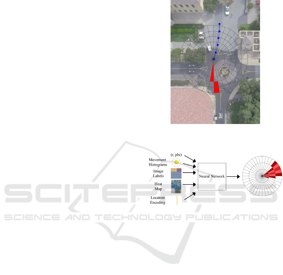
Figure 1: Example of a radial grid centered on the last ob-
served position of a road user illustrated on image from the
Stanford Dataset (Robicquet et al., 2016).
Figure 2: Input and Output Structure of the Network.
given position. By counting directional statistics over
time, continuous learning is possible. Furthermore, a
heat map indicating which areas in the environment
are likely to be walked on by pedestrians is also used.
In order to be able to apply the prediction sys-
tem without any data from this intersection, mod-
els should be transferable. This is done by learning
a movement model of pedestrians at intersections in
general from multiple dataset from arbitrary intersec-
tions.
Finally, the model should be able to continuously
learn and improve its prediction capability. For that,
we propose continuously improving by updating in-
put features of e.g. the input features containing in-
tersection specific patterns.
All those input features are then combined into
one LSTM-based NN model (see Fig. 2). The grid
map-based approach by Kim et al. and Park et al. is
promising for a model capturing the uncertainty of its
prediction since it is possible to represent options of
action (Kim et al., 2017) (Park et al., 2018). Thus, a
local grid map, centered on the observed pedestrian is
the output of the network (see Fig. 1).
Continuously Improving Model of Road User Movement Patterns using Recurrent Neural Networks at Intersections with Connected Sensors
321

4 IMPLEMENTATION
Within this chapter, details about the implementation
of the presented prediction model concept are given.
Due to the use of a grid map as prediction output,
an euclidean distance metric is not directly applica-
ble and new metrics are needed. Thus, new metrics
for evaluating grid maps are proposed in this chapter.
4.1 Data Preprocessing
The first step of data preprocessing is a resampling
step to a sample rate of 2.5 Hz. After splitting the
sequence in a training and a test set with a relation
of 80:20, the sequences are enriched by additional in-
put features. Then, the sequences are separated into
input and output snippets, where an input length of
10 steps and an output length of six steps is chosen.
This corresponds to four seconds of observation and
a prediction horizon of 2.4 seconds. The input trajec-
tories of the training and the test set are normalized
sequence-wise to have a mean of zero and a variance
of one.
4.2 Transferability
To ensure transferability of the model, the input se-
quences cannot be in Cartesian coordinates. If they
were, the network would most likely overfit based on
trajectories which it would see often. This would, for
example, happen in a scene, where there is a very
crowded entrance attracting many pedestrians. Trans-
ferring the model learned on this data to another in-
tersection would result in predicting trajectories in the
same area as if there were a similarly crowded area.
Since this is something to prevent, the coordinates
must not be absolute but rather relative ones, which
is done by converting the input trajectory coordinates
to relative polar coordinates.
4.3 Static Environment
Static map data is different for every intersection but
does not contradict the requirement of transferability
since static map information can easily be created for
every intersection. For the static map, four different
labels are applied to the scene, which results in the
colored image in Fig. 3. Red encodes buildings and
solids, Blue represents streets, Violet grass, bushes or
trees and Yellow indicates sidewalks. The values of
the different areas are used as input for the network
in a nine-dimensional vector. This vector includes the
label of the current position and the labels of the sur-
roundings in eight directions. For every direction, the
Figure 3: Retrieval of surrounding static map data(image
labels).
mean label of the corresponding area is calculated,
where the size of the area can be parameterized. I.e.,
if the label of direction 3 with an area size of 3 by 3
in Fig. 3 should be calculated, the center of the upper
middle quadrant is chosen.
4.4 Dynamic Environment
Besides the static environment, the dynamic environ-
ment needs to be considered. As only pedestrians and
bicyclists are contained in the used dataset, only these
traffic participants are taken into account. As a sim-
ple representation, an occupancy grid-map containing
how many people are around a given person at a par-
ticular time step is calculated. For every time step,
a grid is initialized over the whole area of the scene,
where the size of each grid cell can be parameterized
and each cell is initialized with zero. Experiments
showed, that the best performing grid cell size is 16
by 16 pixels. To fill the grid for every time step, the
value in a cell in a grid for a particular time step is
increased by one if and only if there is an observed
traffic participant at this time step in this cell.
As a more sophisticated alternative to the sim-
ple occupancy grid map, another representation was
built. Since the occupancy gridmap only captures how
many other traffic participants are in a certain direc-
tion, basically three important pieces of information
are missing: the distance, movement direction and
velocity of those road users. Our proposed solution
to this is the encoding of the surroundings using an
autoencoder (Bengio et al., 2013). Similarly to the
time step-indexed map used for the occupancy grid,
the same matrix structure is created. However, in-
stead of creating one matrix for every time step, only
one matrix for every five time steps is used, which
encodes the information of all time steps. This leads
to one matrix representing the positions of every traf-
fic participant currently on the scene during five time
steps. This makes it possible to capture movements in
VEHITS 2019 - 5th International Conference on Vehicle Technology and Intelligent Transport Systems
322

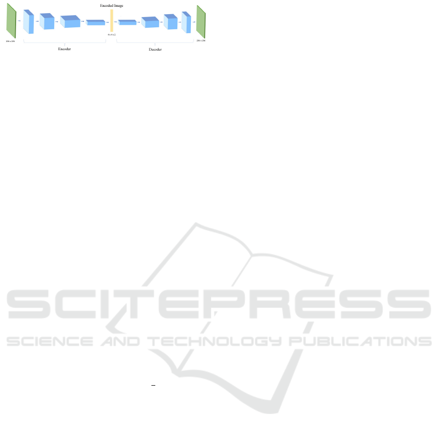
Figure 4: Autoencoder structure.
a small matrix. The resolution of the positions on the
scene is scaled down by half. As structure of the au-
toencoder, a Convolutional Neural Network (CNN)-
autoencoder is chosen, which reduces the input di-
mension of 256 by 256 to a representation of 4 by
4 by 2 and then back to 256 by 256. The structure of
the autoencoder can be seen in Fig. 4.
During preprocessing the data, for every step in
the trajectory, the current surroundings of the corre-
sponding traffic participant are calculated. This image
of the surroundings in the size of 256 by 256 pixels
are then passed into the saved encoder. The result is
a 32-dimensional representation of the surroundings,
which includes the paths of every other road user in
the area during the last five time steps.
4.5 Intersection-specific Patterns
There are two kinds of intersection-specific patterns,
which are used in the model: Firstly, statistical his-
tograms counting how many people are going to
which direction from the current position. Secondly a
heat map, which resembles at which positions at the
intersection pedestrians are often present.
For the movement direction histograms, the pos-
sible directions are reduced to eight directions, i.e.,
every direction has a range of 45 degrees. The ini-
tial directional movement values are
1
8
, because the
chance to go in the eight different directions from the
current position is the same for every direction. The
corresponding data structure contains a matrix with as
many rows and columns as there are pixel in the scene
image. Every cell represents a pixel P in the scene and
contains an eight-dimensional vector V , where, for
every direction D1 - D8, the number of traffic partic-
ipants going into this direction on average from point
P is saved. The size of the area which is recognized as
one direction is parametrizable. Experiments showed
that the best performing size is 16 by 16 pixels. This
leads to a data structure, which holds a histogram over
eight movement directions from any given point on
the scene.
The heat map is built as a matrix in the size of the
intersection scene in pixels. Every cell of this matrix
represents a position a traffic participant can have in
the scene. To fill this matrix, a counter starting at zero
is increased whenever a person in the scene appeared
at that cell. During the preprocessing, the position P
of the currently observed traffic participant is calcu-
lated with regard to the chosen cell size of the heat
map. Similarly to the occupancy grid map, the heat
map values in eight directions from the position P are
extracted from the datastructure.
Both input features support the requirement of
continuous learning, because they can be improved
over time by updating the statistics using the newly
observed data.
4.6 Gridmap Output
Because the input trajectory is represented in polar
coordinates, the grid maps used as output are radial
polar coordinate grids. A resolution of five degrees is
chosen for the angle, and a resolution of five to one is
chosen for the radius.
Implementation-wise, the label is represented as a
matrix. Every row represents an angle of five degrees,
and every column represents a radius of four pixels,
which results in a dimension of 72 by 80. The 80
columns come from approximating the maximum dis-
tance of a traffic participant during the prediction time
to less or equal to 400 pixels. The conversion factor
from pixels to meters is 0.037 for the used dataset,
which equals in a maximum distance of 14.8 meters
during 2.4 seconds. This corresponds to a speed of
around 22 km/h, which we consider as sufficient for
pedestrians.
4.7 Neural Network Model
The Neural Network model is implemented using
Keras (Chollet et al., 2015). In the proposed model,
Gated Recurrent Units (GRUs), a variant of Recurrent
Neural Networks (RNNs) similar to LSTMs are used.
Our best performing model consists of two dense
layers and three stacked GRUs layers. The input
of the network represents a masking layer to allow
short observations as input. After this masking layer
there are three stacked GRU layers with 128 neurons
each. Tanh is used as an activation function and a
hard sigmoid is used as a recurrent activation func-
tion.
After the GRU layer, there are two fully connected
layers with the first consisting of 16 neurons with a
relu activation function. The second fully connected
layer is the output layer of the network. It consists of
5760 neurons, which equals to the dimensions of the
grid map labels. The sigmoid function is chosen as an
activation function for this layer.
The model was trained using the Adam extension
AMSGrad for 200 epochs. As error function the cat-
egorical crossentropy function is chosen.
Continuously Improving Model of Road User Movement Patterns using Recurrent Neural Networks at Intersections with Connected Sensors
323

4.8 Metrics
For evaluation, new metrics were necessary. Thus,
we propose the metrics Mean Overlapping Percent-
age (MOP), Partwise Overlapping Percentage (POP),
Mean Percentage (MP) and Wrong Percentage (WP)
metric. The Combined Metric Value (CMV) com-
bines all presented metrics in one rating value.
The Categorical Cross Entropy Error (CCE) met-
ric is used to capture the difference between the cor-
rect label for one input trajectory and the output of the
model.
− Σx
true
× log(x
pred
) (1)
It is calculated as a sum of the discrepancy of all la-
bels with their corresponding model outputs.
The Mean Overlapping Percentage (MOP) metric
is used to capture how much of the true trajectories
are completely overlapped by the output grid map on
average. For every correct label (x
true
i
) it is checked,
if every position marked with a one in the label has a
corresponding probability value in the model predic-
tion (x
pred
i
), which is higher than the threshold. If this
is true for all positions in the label, the label is com-
pletely overlapped. If this is wrong for at least one
of the positions, the complete label is not overlapped.
This metric punishes a prediction which is incorrect
but can be bypassed by always predicting a very high
percentage for every grid map cell. Getting a high
score in this metric should ensure, that all true tra-
jectories are predicted but also, that multiple different
movement options are predicted.
The Partwise Overlapping Percentage (POP) met-
ric captures, how much of each true trajectory is over-
lapped by the model output on average. For every
label, it is checked if the model output overlaps ev-
ery point. If the corresponding position in the model
output grid map has a probability value greater than a
threshold, it is marked with a one, else it is marked
with a zero. Then the average for each label sep-
arately is calculated and afterward the average over
all averages. This metric also punishes wrong pre-
dictions but gives greater insights into how good the
prediction actually is. Similarly to the MOP metric in
can be bypassed by always predicting an occupancy
probability of 100 % for every cell in the output.
The Mean Percentage (MP) metric calculates what
the average chance of occupancy for the correct po-
sitions is. This metric ensures the exactness of the
prediction by punishing the prediction of cells, which
are near but not exactly the right ones. Once again it
can be bypassed by always predicting the occupancy
probability of all cells with 100%.
To counter the bypassing capabilities of the MOP,
POP and MP metric, the Wrong Percentage (WP)
metric is used. This metric captures the average dif-
ference of the true label and the prediction. Simi-
larly to the Kalman filter predictions, the labels for
this metric are enhanced by applying a 3 by 3 discrete
Gaussian filter onto every cell marked with a one in
the label. The metric then subtracts the correct prob-
ability value for every cell from the probability value
the model predicted. This is done for every label and
is averaged afterward. This metric heavily punishes
wrong predicted cells and is a counterweight to the
last three metrics. Since it also not wanted, that only
the, for the model, single correct trajectory is pre-
dicted but instead also different movement options at
the same time, this cannot be the only metric but it
has to be combined with all the other metrics.
This is done by the last metric, the Combined Met-
ric Value (CMV). This metric combines all presented
metric in one rating value. The higher the value is, the
better the prediction behaves while computing pre-
dictions of different movement options but also not
assigning too high occupancy probabilities to all the
cells in the grid map.
(MOP + POP + MP)

CCE
100
+W P ×10

(2)
The value for the CCE metric is scaled down since
it can range between zero and ∞, while the value for
the WP metric is scaled up since it normally ranges
between 0 and 0.005. Furthermore, its influence to
rating the model is crucial as a counterweight to the
MOP, POP and MP metrics. In addition to that, the
MOP, POP, and MP metrics are calculated stepwise.
I.e., those metrics are not only calculated for every
complete trajectory but also separately for every first
step of the trajectory, the first two steps of it and so on.
This captures the decreasing capabilities of the model
for predictions over a longer prediction horizon.
5 RESULTS
For evaluation, a traditional linear Kalman filter is
used, which is a common practice in literature. As
dataset the DeathCircle scene of the Stanford Drone
dataset is used (Robicquet et al., 2016).
The proposed model was amongst other things
evaluated with regard to additional information im-
proving the prediction capabilities. To evaluate this,
seven different stages of additional input features
were compared:
1. Only relative polar coordinates
2. As in 1. plus static map data
VEHITS 2019 - 5th International Conference on Vehicle Technology and Intelligent Transport Systems
324

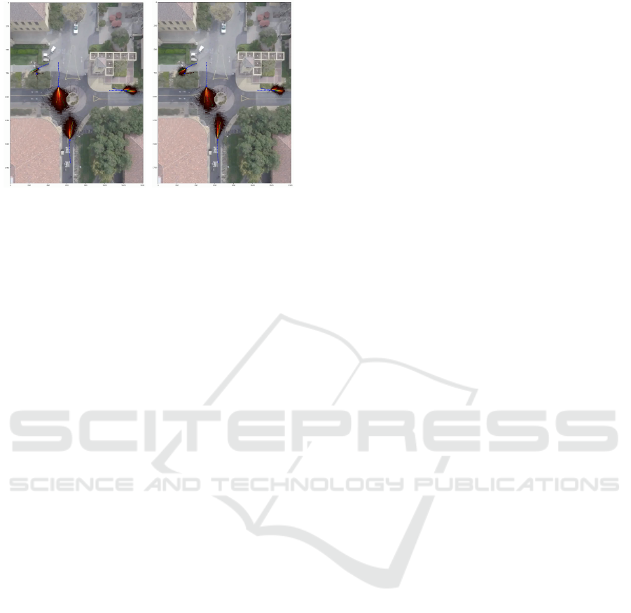
(a) Model with naive grid (b) Model with encoding
Figure 5: Comparison of the Model Prediction.
3. As in 2. plus histograms
4. As in 3. plus naive occupancy grid
5. As in 4. plus heat map
6. As in 5. plus x,y coordinates
7. As in 5. but with encoded surroundings instead of
naive occupancy grid
The first evaluated model reaches a CMV value of
10.879. Especially the CCE value is with 11.056 rel-
atively high, while the WP error is with 0.00227 ex-
tremely low. However, already adding the static map
data as additional input features improves the CMV
value to 11.330. The CCE value is lowered to 9.482,
but also the WP increases to 0.00477. However, all
of those first six models are inferior to the model us-
ing all the additional input features but replacing the
naive occupancy grid approach with the encoded local
surroundings and the basic x,y coordinates. This re-
sults in a CMV of 11.790 with a CCE value of 9.450
and a WP value of 0.00434, where all those values
are highly significantly better than their prior coun-
terparts. This is also achieved when evaluating the
already trained network with smaller fractions of the
sequences with regard to the histograms and the heat
map. Especially the CMV decreases from 11.790 to
8.248 while only using 10 % of the sequences.
In Fig. 5 two different models are compared qual-
itatively. In each picture, the blue dotted line repre-
sents the observed trajectory, the green one denotes
the true future trajectory, the yellow line indicates the
prediction of the Kalman filter, and the heat map in
red describes the model output. The prediction for the
trajectory entering the roundabout from above con-
tains more possible movement options for the right
than for the left model. This is for this specific area a
valid result since it is possible that, even while ap-
proaching the roundabout in a very straightforward
manner, the traffic participant will turn and leave the
roundabout in westward direction. This is also a dif-
ference for the road user arriving at the roundabout
from underneath. The prediction depicted on the left
already predicts a possible left or right turn, but the
roundabout is yet relatively far away. The prediction
of the right model makes for this position a lot more
sense.
Furthermore, the model using the naive grid tends
to learn a cross-shaped prediction for traffic partici-
pants not moving. This can be seen on the right for the
pedestrian at position (250, 750) next to the arriving
pedestrian. This form of prediction does not happen
for the model using the Encoding. The predictions
of the two pedestrians on the right side of the image
and the walking pedestrian at position (250, 700) are
equally good in both models.
6 CONCLUSIONS
In this paper, we presented a new approach to predict
trajectories, which at the same time captures the un-
certainty in prediction by a polar grid map, is trans-
ferable to other intersections, considers static and
dynamic environment information as well as scene-
specific patterns and is able to improve continuously
over time with new measurement data without re-
training the model.
The proposed model was evaluated via different
metrics and compared for different sets of input fea-
tures and also with the basic Kalman filter prediction
approach. This evaluation resulted in a significantly
better prediction when using the proposed set of input
features, containing relative polar coordinates, static
map data, movement histograms, a movement heat
map, an encoding of the surrounding traffic partici-
pants and the plain Cartesian coordinates. Our re-
sults show significantly better scores for all intro-
duced metrics compared to the Kalman filter, which
is supported by qualitative evaluations.
We plan to enhance the proposed model in the fu-
ture by an improved encoding of the dynamic envi-
ronment. Furthermore, we plan to create a statistical
baseline model for predictions with grid maps as out-
put based on measurement data from intersections.
ACKNOWLEDGEMENTS
The work for this paper was partially funded within
the project I2EASE funded by the German Federal
Ministry of Education and Research based on a deci-
sion of the German Federal Diet.
Continuously Improving Model of Road User Movement Patterns using Recurrent Neural Networks at Intersections with Connected Sensors
325

REFERENCES
Alahi, A., Goel, K., Ramanathan, V., Robicquet, A., Fei-
Fei, L., and Savarese, S. (2016). Social LSTM: Hu-
man trajectory prediction in crowded spaces. In 2016
IEEE Conference on Computer Vision and Pattern
Recognition (CVPR). IEEE.
Bartoli, F., Lisanti, G., Ballan, L., and Del Bimbo, A.
(2017). Context-aware trajectory prediction. arXiv
preprint arXiv:1705.02503.
Bengio, Y., Courville, A., and Vincent, P. (2013). Represen-
tation learning: A review and new perspectives. IEEE
Transactions on Pattern Analysis and Machine Intel-
ligence, 35(8):1798–1828.
Bock, J., Beemelmanns, T., Kl
¨
osges, M., and Kotte, J.
(2017). Self-learning trajectory prediction with recur-
rent neural networks at intelligent intersections. In
Proceedings of the 3rd International Conference on
Vehicle Technology and Intelligent Transport Systems.
Chollet, F. et al. (2015). Keras. https://github.com/
fchollet/keras.
Goldhammer, M., Doll, K., Brunsmann, U., Gensler, A.,
and Sick, B. (2014). Pedestrian’s trajectory forecast in
public traffic with artificial neural networks. In 2014
22nd International Conference on Pattern Recogni-
tion. IEEE.
Hatfield, J. and Murphy, S. (2007). The effects of mobile
phone use on pedestrian crossing behaviour at sig-
nalised and unsignalised intersections. Accident Anal-
ysis & Prevention, 39(1):197–205.
Hug, R., Becker, S., H
¨
ubner, W., and Arens, M. (2018).
Particle-based pedestrian path prediction using lstm-
mdl models.
Kim, B., Kang, C. M., Lee, S., Chae, H., Kim, J., Chung,
C. C., and Choi, J. W. (2017). Probabilistic vehicle
trajectory prediction over occupancy grid map via re-
current neural network. CoRR, abs/1704.07049.
Kim, S.-W., Chong, Z. J., Qin, B., Shen, X., Cheng, Z., Liu,
W., and Ang, M. H. (2013). Cooperative perception
for autonomous vehicle control on the road: Motiva-
tion and experimental results. In 2013 IEEE/RSJ In-
ternational Conference on Intelligent Robots and Sys-
tems. IEEE.
Lerner, A., Chrysanthou, Y., and Lischinski, D. (2007).
Crowds by example. In Computer Graphics Forum,
volume 26, pages 655–664. Wiley Online Library.
Park, S., Kim, B., Kang, C. M., Chung, C. C., and Choi,
J. W. (2018). Sequence-to-sequence prediction of ve-
hicle trajectory via lstm encoder-decoder architecture.
arXiv preprint arXiv:1802.06338.
Pellegrini, S., Ess, A., Schindler, K., and van Gool, L.
(2009). You ll never walk alone: Modeling social be-
havior for multi-target tracking. In 2009 IEEE 12th
International Conference on Computer Vision. IEEE.
Pfeiffer, M., Paolo, G., Sommer, H., Nieto, J. I., Siegwart,
R., and Cadena, C. (2017). A data-driven model for
interaction-aware pedestrian motion prediction in ob-
ject cluttered environments. CoRR, abs/1709.08528.
Rauch, A., Klanner, F., Rasshofer, R., and Dietmayer, K.
(2012). Car2x-based perception in a high-level fu-
sion architecture for cooperative perception systems.
In 2012 IEEE Intelligent Vehicles Symposium. IEEE.
Robicquet, A., Sadeghian, A., Alahi, A., and Savarese, S.
(2016). Learning social etiquette: Human trajectory
understanding in crowded scenes. In European con-
ference on computer vision, pages 549–565. Springer.
Schnieder, L., Knake-Langhorst, S., and Gimm, K. (2016).
AIM research intersection: Instrument for traffic de-
tection and behavior assessment for a complex urban
intersection. Journal of large-scale research facilities
JLSRF, 2.
van Arem, B., van Driel, C. J. G., and Visser, R. (2006).
The impact of cooperative adaptive cruise control on
traffic-flow characteristics. IEEE Transactions on In-
telligent Transportation Systems, 7(4):429–436.
Varshneya, D. and Srinivasaraghavan, G. (2017). Human
trajectory prediction using spatially aware deep atten-
tion models. arXiv preprint arXiv:1705.09436.
WHO (2016a). Developing global targets for road safety
risk factors and service delivery mechanisms. http:
//www.who.int/violence_injury_prevention/
road_traffic/road-safety-targets/en/ [ac-
cessed in February 2019].
WHO (2016b). Global status report on road safety
2015. http://www.who.int/violence_injury_
prevention/road_safety_status/2015/en/ [ac-
cessed in February 2019].
VEHITS 2019 - 5th International Conference on Vehicle Technology and Intelligent Transport Systems
326