
2D-STR: Reducing Spatio-temporal Traffic Datasets by Partitioning and
Modelling
Liam Steadman
1
, Nathan Griffiths
1
, Stephen Jarvis
1
, Stuart McRobbie
2
and Caroline Wallbank
2
1
Department of Computer Science, University of Warwick, Coventry, CV4 7AL, U.K.
2
TRL, Wokingham, RG40 3GA, U.K.
Keywords:
Spatio-temporal Data, Data Reduction, Data Partitioning.
Abstract:
Spatio-temporal data generated by sensors in the environment, such as traffic data, is widely used in the
transportation domain. However, learning from and analysing such data is increasingly problematic as the
volume of data grows. Therefore, methods are required to reduce the quantity of data needed for multiple types
of subsequent analysis without losing significant information. In this paper, we present the 2-Dimensional
Spatio-Temporal Reduction method (2D-STR), which partitions the spatio-temporal matrix of a dataset into
regions of similar instances, and reduces each region to a model of its instances. The method is shown to be
effective at reducing the volume of a traffic dataset to <5% of its original volume whilst achieving a normalise
root mean squared error of <5% when reproducing the original features of the dataset.
1 INTRODUCTION
Spatio-temporal data generated by sensors in the en-
vironment is used widely in many domains. In the
transportation domain, traffic data measures the speed
and flow of a traffic network at a specific location and
time. Analysing and learning from traffic data allows
us to understand the relationship between different
roads or areas of a road network, as well as understand
the temporal characteristics of the network. Common
tasks in analysing traffic data include: (i) imputing
missing instances, instances between sensors or time
intervals; (ii) identifying unusual behaviours, such as
sensors that perform unexpectedly or periods of time
wherein instances do not fit expected trends; (iii) cal-
culating statistics, such as high and low values for a
time period or calculating the variance within a time
period from the expected trend; (iv) comparing time
periods or sensors, for example performing a month-
on-month time series analysis; and (v) predicting fu-
ture instances.
The volume of traffic data in the transportation
domain has increased significantly in recent years,
and this presents several challenges for data scien-
tists. Processing larger spatio-temporal datasets re-
quires more processing time and is sometimes infea-
sible entirely. Therefore, methods are required to re-
duce the volume of the data to be processed whilst
minimising the error introduced in later analysis or
modelling. The aim is not necessarily to compress the
data, since this may require decompression before the
data can be used again. Rather, we aim to summarise
the data in a manner such that analysis and processing
can be performed directly on the summarised data.
In this paper, we propose a new dataset reduc-
tion method, 2-Dimensional Spatio-Temporal Reduc-
tion (2D-STR), for decreasing the volume of a traffic
dataset whilst minimising the information lost in the
process. The method uses the variance within the data
to partition the dataset, then models each resulting re-
gion using an appropriate modelling technique. The
algorithm iteratively trades information loss for quan-
tity of data output until an objective function is min-
imised. 2D-STR is designed to be extensible given the
uses of the reduced dataset in further analysis, and is
evaluated using data recorded from traffic count sen-
sors within a motorway network in England.
The remainder of this paper is structured as fol-
lows. Section 2 reviews existing methods for reduc-
ing the volume of a traffic dataset. Section 3 for-
malises the problem to be solved and introduces the
notation used in this paper, and Section 4 describes
the proposed data reduction method. Sections 5 and
6 evaluate the effectiveness of 2D-STR on a set of
traffic datasets taken from locations in England and
compares it with other techniques. Finally, Section 7
concludes the paper and gives some future directions
of the work.
Steadman, L., Griffiths, N., Jarvis, S., McRobbie, S. and Wallbank, C.
2D-STR: Reducing Spatio-temporal Traffic Datasets by Partitioning and Modelling.
DOI: 10.5220/0007679100410052
In Proceedings of the 5th International Conference on Geographical Information Systems Theory, Applications and Management (GISTAM 2019), pages 41-52
ISBN: 978-989-758-371-1
Copyright
c
2019 by SCITEPRESS – Science and Technology Publications, Lda. All rights reserved
41

2 RELATED WORK
It is often infeasible to process a spatio-temporal
dataset in its raw form because of the volume of data
present. Therefore, several techniques exist for re-
ducing the quantity of data in order to facilitate faster
modelling and analysis. In this section, we give an
overview of existing methods for achieving this aim.
2.1 Selection and Engineering of
Features and Instances
Many existing methods for reducing datasets focus on
removing or retaining a subset of features or instances
from the original dataset. Feature selection tech-
niques can be separated into three categories. First,
filter methods rank features in the dataset according
to a relevancy criterion, such as Shannon entropy,
and remove any features which score below a defined
threshold. Second, wrapper methods use search al-
gorithms to find the optimal subset of features ac-
cording to an objective function. The third category,
embedded methods, incorporate feature selection as
part of the training process of machine learning tech-
niques. Several feature selection techniques for real-
valued data exist, and a number of reviews of these
can be found in related literature (Xue et al., 2016; Li
et al., 2017). Similar to feature selection, instance se-
lection techniques have been surveyed in the context
of different application domains (Garcia et al., 2012;
Acampora et al., 2016; Mukahar and Rosdi, 2018).
In contrast to selection techniques, feature engi-
neering techniques (often referred to as feature ex-
traction) project the original features of a dataset
onto a new feature space, often of a differing dimen-
sionality. Some feature engineering techniques map
the original dataset onto a smaller set of engineered
features, thus reducing the volume of the dataset.
The best mapping is that which optimises an objec-
tive criterion, such as explained variance or accu-
racy when combined with modelling. Feature extrac-
tion methods can be grouped into linear algorithms,
such as Principal Components Analysis (PCA) (Pear-
son, 1901) and Linear Discriminant Analysis (LDA)
(Martinez and Kak, 2001), and non-linear algorithms,
such as Isomap and Locally Linear Embedding (LLE)
(Tenenbaum et al., 2000; Roweis and Saul, 2000).
Instance engineering techniques (often referred to
as feature abstraction or prototyping) create a smaller
set of prototype instances which represent the origi-
nal instances. Prototyping has been shown to be ef-
fective in reducing the size of training sets required
for tasks such as k-Nearest Neighbour classification
(Ougiaroglou and Evangelidis, 2012).
Whilst effective at reducing the volume of a
dataset, feature and instance selection techniques may
remove data and patterns that are significant for sub-
sequent analysis. They fail to capture the spatial and
temporal nuances of the data and require the user
to have knowledge of the modelling or analysis they
will perform ahead of time. Instead, it may be more
beneficial to retain information about all features and
instances. Furthermore, the features output by ex-
traction techniques are often incomprehensible to hu-
mans and require mapping back to the original fea-
ture space. The instances resulting from instance en-
gineering may not exist in the original dataset and this
may cause problems in later processing. Finally, se-
lection and engineering techniques do not take advan-
tage of the spatio-temporal correlations in the data.
2.2 Data Sketching
Data sketching techniques create query-specific sum-
maries using a fixed number of passes over the data.
Many of these techniques require just one pass over
the data and so are very fast to compute.
Many sketching techniques focus on counting
items, such as the Count-Min sketch and its adap-
tation for real-valued data (Cormode and Muthukr-
ishnan, 2005; Sisovic et al., 2018), and determining
membership, such as the Bloom Filter (Bloom, 1970).
Other techniques, such as the HyperLogLog (HLL)
algorithm, focus on answering cardinality queries
(Flajolet et al., 2007). Most sketching techniques do
not consider the spatial and temporal nature of the
data and do not support analysis questions such as
those presented in Section 1.
In the spatio-temporal domain, methods have been
proposed that combine instance selection data sketch-
ing with the Kalman filter to track large-scale spatio-
temporal processes (Berberidis and Giannakis, 2015;
Berberidis and Giannakis, 2017). Furthermore, Tai et
al. presented a sketching method for building linear
classifiers over a spatio-temporal dataset (Tai et al.,
2018). This method destroys features which are not
heavily weighted by the linear classifier and so pre-
vents analysis of all features. Sketching techniques
are still limited in the analyses or later modelling they
support (Cormode et al., 2012). They are created
specifically for particular queries and since the origi-
nal dataset is destroyed after the sketch is created, it
is not possible to recreate the data for other analyses.
2.3 Data Reduction by Modelling
Whilst the techniques discussed above result in the
loss of instances or features, some techniques have
GISTAM 2019 - 5th International Conference on Geographical Information Systems Theory, Applications and Management
42

been investigated for reducing a dataset using statis-
tical modelling. The IDEALEM algorithm partitions
a data stream into blocks of a fixed size (Wu et al.,
2017). Key statistical properties about these blocks,
such as min, max and average values, are then used
to identify similar blocks which can be reduced to
the same model. By processing each of its proto-
type blocks, IDEALEM allows us to identify unusual
temporal periods that do not fit expected trends. In
the same way, generating statistics over the stream is
faster when compared to processing the raw dataset.
IDEALEM also enables an element of time series
analysis and comparison of different sensors or time
periods. However, since prototype blocks are retained
in the form of raw data, and the method only consid-
ers the temporal nature of spatio-temporal data, IDE-
ALEM does not permit spatio-temporal imputation.
Similar to IDEALEM, the ISABELA algorithm
partitions each feature into fixed size spatial windows
and sorts the instances into ascending order within
each window (Lakshminarasimhan et al., 2011). A
B-spline curve is then fitted to each window and the
parameters for the curve of each window stored us-
ing temporal encoding. ISABELA permits the gener-
ation of statistics for given temporal and spatial pe-
riods, provided that those periods cover the spatial
and temporal windows used by ISABELA exactly
and, in the same way, partially permits identifying un-
usual spatio-temporal regions. However, since the in-
stances in each window are stored in ascending order
by value, a mapping from this ordering to the tem-
poral ordering also needs to be stored. Many sensor
datasets, such as traffic datasets, are more smooth and
cyclic than the scientific data ISABELA was designed
for, and so can be modelled effectively without need-
ing to be sorted (Birvinskas et al., 2012).
Deep autoencoders have also been used to model
the temporal features of spatio-temporal datasets
(Wang et al., 2016). The Sparse Autoencoder (SAE)
has been used to reliably estimate missing data in
spatio-temporal sensor datasets (Wong et al., 2014).
This fitting of a summary, which minimises the root
mean square error (RMSE) over instances in both the
discrete spatial and temporal dimensions, is able to
impute missing values given other instances from the
same time. It may be possible to adapt this approach
to incorporate multiple time instances, e.g. the whole
dataset, and store the autoencoder weights for the pur-
poses of reproducing the dataset. However, autoen-
coder weights can be difficult to interpret and so pre-
vent manual analysis of the reduced dataset.
In the domain of traffic dataset analysis, Pan et al.
have proposed a two-part algorithm that summarises
a spatio-temporal traffic sensor dataset (Pan et al.,
2010). Their method creates a spatio-temporal signa-
ture of the dataset using a technique such as wavelet
decomposition, and probabilistically stores separately
the outliers that fall outside an acceptable error mar-
gin of this signature. Whilst this technique accounts
for the cyclic and seasonal natures of traffic data, it
performs poorly in reducing regions containing many
outliers. For example, instances from national hol-
idays (temporal domain) and areas of construction
work (spatial domain) which are known to break reg-
ular traffic cycles will be labelled as outliers. There-
fore, such instances will need to be stored in their raw
form thereby hindering the reduction of data volume.
The algorithm permits analysis of unusual periods, by
examining the signatures and outliers of the period,
comparison of time series, and statistics to be gener-
ated from the data in its reduced format.
In our review of literature these are the only ex-
amples of reduction by modelling for spatio-temporal
data, and the technique presented by Pan et al. is the
only example for traffic data. This suggests that the
topic of reducing a dataset to a set of spatio-temporal
regions and models has yet to be explored deeply.
3 SPATIO-TEMPORAL DATASET
REDUCTION
Many spatio-temporal datasets, such as traffic
datasets, contain spatial areas and temporal periods
which exhibit low amounts of change. That is, the
instances within these areas and periods have low
variance when compared to the variance of the entire
dataset. For example, a traffic sensor may record sim-
ilar average speeds and vehicle counts for several con-
secutive 15-minute windows throughout the day. To
decrease the quantity of data to be analysed or mod-
elled in these cases, we can group similar consecutive
instances together to form spatio-temporal regions in
which the data exhibits low variance. We do not wish
to lose information of any features, sensors or time in-
tervals, however we do wish to decrease the quantity
of data present in the resulting dataset. It is desirable
to support many types of analysis or modelling, and
multiple passes of the dataset are permitted. By iden-
tifying regions of similar instances in the dataset and
reducing these regions to models, these requirements
are met. The nuances of the original instances can
be maintained and answering queries on the dataset is
still supported. This section formalises this approach
and the notation used in this paper.
A traffic dataset D is a set of instances in the T × S
space, where T is a set of discrete time intervals and
S is a discrete set of spatially fixed sensors along the
2D-STR: Reducing Spatio-temporal Traffic Datasets by Partitioning and Modelling
43

road. We assert that D may contain missing instances,
i.e |D| ≤ |T | · |S|, and that T and S are ordered, thus it
is possible define ranges over them. We can view D as
a 2-dimensional matrix (Figure 1(a)), where columns
represent the ordered set of discrete sensors and rows
represent the ordered set of discrete time intervals. By
permitting missing instances we also allow for sen-
sors to be asynchronous.
Each instance d
t,s
is a vector of values over F ∈
N features, d
t,s
= (d
t,s
(1),...,d
t,s
(F)). For example,
these features may be vehicle count and average vehi-
cle speed. In this work, for the purposes of generality,
we assume the non-referencing features in D are real-
valued. Thus, D : T × S → R
F
. Techniques exist for
representing binary and categorical features as real-
valued data, and appropriate clustering algorithms can
be used for binary and categorical features.
We wish to find the set R of non-overlapping re-
gions in the T × S space, where each region R
i
is a
rectangle (Figure 1(d)). Each region R
i
has a defined
beginning and ending time, t
b
and t
e
, and a beginning
and ending sensor, s
b
and s
e
. Furthermore, we use r
i
to denote the subset of instances from dataset D that
belong to region R
i
, r
i
= {d
t,s
∈ D|t
b
≤ t ≤ t
e
,s
b
≤ s ≤
s
e
: (t
b
,t
e
,s
b
,s
e
) = R
i
}.
Each region R
i
is associated with a model M
i
which is fitted to the instances r
i
. The reduction uses
a single modelling technique, which is able to charac-
terise the spatio-temporal nuances of the dataset, for
all models. We refer to the set of summary models in
the reduction as M = (M
1
,...,M
|R|
), and denote |M
i
|
to be the number of coefficients used to store model
M
i
. Finally, we use the term reduction to refer to a
pair of regions and their models (R, M). The notation
used in this paper is summarised in Table 1.
In reducing D to (R, M) we wish to minimise the
information lost. We refer to the information lost
by reducing D to reduction (R,M) as e(D,(R,M)).
One method of measuring information loss is to recre-
ate the dataset as D
0
using the set of region models
(R,M), and then use an appropriate measure of the
difference between each instance in D and its corre-
sponding instance in D
0
, i.e. e(D,(R,M)) = e(D,D
0
).
A simple example is the Mean Absolute Percentage
Error (MAPE) averaged across the dataset:
e
MAPE
(D,D
0
) =
1
|D| · F
∑
d
t,s
∈D
F
∑
j=1
d
t,s
( j) − d
0
t,s
( j)
d
t,s
( j)
(1)
An alternative measure is the Normalised Root
Mean Square Error (NRMSE) averaged across the
dataset:
e
NRMSE
(D,D
0
) =
1
F
F
∑
j=1
ψ( j,D,D
0
)
range( j)
(2)
Table 1: Notation used in this paper.
Symbol Definition
D Original dataset over the discrete or-
dered set of time intervals T and set
of sensors S
F The number of real-valued features
in D, excluding the referencing fea-
tures T and S
d
t,s
An individual instance in D
d
t,s
( j) Value of d
t,s
for feature j
R A set of non-overlapping spatio-
temporal regions on D
R
i
An individual spatio-temporal re-
gion in R
r
i
Set of instances of dataset D con-
tained in region R
i
M Set of summary models belonging to
regions R of dataset D
M
i
Summary model of region R
i
, fitted
over the instances r
i
, with the num-
ber of coefficients used to store M
i
represented as |M
i
|
(R,M) A reduction of dataset D
e(D,(R,M)) Error introduced after D is reduced
to regions R and their models M
q(D,(R,M)) Ratio of storage required for regions
R and summary models M compared
to the original dataset D
h(D,(R,M)) Objective function used to find the
best reduction given parameter α,
the constant that prioritises between
e(D,(R,M)) and q(D,(R,M))
where,
ψ( j,D,D
0
) =
s
∑
t∈T
∑
s∈S
(d
t,s
( j) − d
0
t,s
( j))
2
|D|
and range( j) = max
t,s
(d
t,s
( j)) − min
t,s
(d
t,s
( j)). It is
preferable to use the MAPE metric when the error of
an instance relative to its original values is important.
Conversely it is preferable to use the NRMSE metric
when the error of an instance relative to the range of
values observed for the feature is preferred.
Whilst minimising the information lost across D,
we also wish to minimise the storage cost of the data.
In the case of the original dataset this is given by the
number of instances multiplied by the number of fea-
tures including the spatial and temporal referencing
features, as shown in Equation 3. In the case of the re-
duced dataset, the data output is a start and end value
of each region in the spatial and temporal dimensions,
along with the coefficients required to store the model
GISTAM 2019 - 5th International Conference on Geographical Information Systems Theory, Applications and Management
44

s
1
s
2
s
3
s
4
s
5
t
1
t
2
t
3
t
4
t
5
(a)
s
1
s
2
s
3
s
4
s
5
t
1
t
2
t
3
t
4
t
5
(b)
s
1
s
2
s
3
s
4
s
5
t
1
t
2
t
3
t
4
t
5
(c)
s
1
s
2
s
3
s
4
s
5
t
1
t
2
t
3
t
4
t
5
(d)
Figure 1: Stages of the hierarchical partitioning technique: (a) the raw data; (b) the data clustered into 4 clusters using
hierarchical clustering (clusters coloured green, yellow, blue and red); (c) rectangles of contiguous clusters are found in the
spatio-temporal feature space; (d) the resulting 8 regions, where instances within each region belong to the same cluster.
for each region. Since a single modelling technique is
assumed to be used throughout the dataset there is no
need to store the modelling technique used. The stor-
age required for a reduced dataset is shown in Equa-
tion 4, and we use the quotient of these two measures
to define the storage ratio, as shown in Equation 5.
storage(D) = |D| · (|F| + 2) (3)
storage((R,M)) =
|M|
∑
i=1
|M
i
| + (4 · |R|) (4)
q(D,(R,M)) =
storage((R,M))
storage(D)
(5)
In data reduction, we require an objective func-
tion that guides the methodology and allows the user
to indicate their preference for the trade-off between
minimising storage cost and information loss. The
objective function used in this paper is the sum of the
information lost and the storage ratio, as used in (Guo
et al., 2012):
h(D,(R,M)) = e(D,R)+αq(D,R) (6)
Here, α is a user-defined constant that weights the
importance of storage cost against information loss.
4 2D-STR
The 2-Dimensional Spatio-Temporal Reduction algo-
rithm, 2D-STR, is an iterative algorithm that begins
with a single rectangular region over the T ×S spatio-
temporal space defined by D. A model, of the lowest
order, is fitted to the instances in this region using a
predefined modelling technique. On each iteration the
algorithm decides whether to partition the T ×S space
into more non-overlapping rectangular regions, or in-
crease the model complexity of one of the existing
regions, thereby aiming to improve its accuracy. The
decision made at each step is that which minimises
the objective function h(D,(R,M)). The function uses
the parameter α to weight the importance of storage
reduction and model accuracy.
4.1 Data Partitioning
To reduce a dataset, 2D-STR first partitions the
dataset into regions of similar instances. Whilst meth-
ods exist for partitioning a dataset, such as quadtree
and octree (Samet, 1984), the number of new parti-
tions introduced by these methods at each level of de-
composition is fixed. Instead, it is more beneficial
to use the variance within the data to determine how
many partitions are introduced at each level. 2D-STR
uses a novel technique, based on the variance within
the data, to partition the data.
First, the instances in the dataset D are clustered
using hierarchical agglomerative clustering in the fea-
ture space (Figure 1(b)). By clustering instances us-
ing the F features in the dataset rather than clustering
in the T × S space, 2D-STR finds instances that have
similar feature values regardless of when and where
the instances were generated. Hierarchical clustering
is used as the clusters found in the feature space are
not expected to be globular and the resultant hierar-
chical tree permits fast retrieval as the number of clus-
ters required changes (Fahad et al., 2014).
After clustering, each instance in the T × S spatio-
temporal matrix is labelled with the cluster it has been
grouped into. To partition the T × S spatio-temporal
matrix into homogeneous rectangular regions, that is
regions containing instances belonging to the same
cluster, a Monte Carlo algorithm is used (Figure 1(c))
(Lemley et al., 2016). On each iteration, the regioning
algorithm randomly chooses an instance from the ma-
trix which has yet to be placed into a region and uses
it as a starting point for a new region. Starting with
this instance and whilst ensuring cluster homogeni-
ety, the algorithm iteratively adds instances with the
same time value from each preceding sensor along
the road to the region. When an instance belonging
2D-STR: Reducing Spatio-temporal Traffic Datasets by Partitioning and Modelling
45

to a different cluster is about to be added to the re-
gion, the algorithm stops adding preceding sensors.
The same action is then repeated for sensors ahead of
the starting instance along the road, and the beginning
and ending time intervals of the region. This results
in rectangular regions of the form depicted in Figure
1(d), and rectangular regions are required to ensure
that the range of each region over space and time can
be easily defined and stored.
As the number of clusters is increased, the hierar-
chical clustering decomposes just one branch of the
cluster tree. As a result, many clusters are unchanged
and retain the same instances. Therefore, the regions
defined for these clusters remain the same. Retaining
regions between iterations is useful as it allows the
models for these regions to persist between iterations.
4.2 Region Modelling
After partitioning D into regions, a technique is re-
quired to model the instances within each region. A
model M
i
is fitted to the instances in each region us-
ing the spatial and temporal values of the instances
in the region as the independent values of the model,
and the values of the real-valued features as depen-
dent values. To maximise the utility of the reduction,
we require the ability to reconstruct the instances of
the dataset after modelling is performed. However, if
the type of analysis to be performed after reduction
is already known and reconstruction is not required,
more appropriate modelling techniques may be used.
In this paper, we consider two illustrative mod-
elling techniques. First, we consider polynomial lin-
ear regression (PLR) because of its ability to ex-
plain traffic sensor data well whilst remaining easy
to interpret and interpolate. Second, we consider
2-dimensional Discrete Cosine Transforms (DCT)
since, like traffic datasets that have been reduced
in previous work (Birvinskas et al., 2012), the traf-
fic data we consider is cyclic and can be explained
well using cosine waves. Each feature is modelled
independently and all features are therefore recon-
structable. In general, the modelling technique used
should allow for variable model complexities, such as
the number of terms used in regression or the number
of coefficients stored for discrete cosine modelling.
4.3 Data Reduction
Before the algorithm can be initiated, a value for α
must be chosen which weights model accuracy, or er-
ror, against the storage ratio in the objective function
(Equation 6). 2D-STR is initiated by partitioning the
instances, as described in Section 4.1, using a single
cluster. Since there is just one cluster, only one region
is created, R
1
. This region is then modelled using the
simplest form of the modelling technique used: in the
case of polynomial regression a polynomial model of
order 0 (simply a mean) is constructed for each fea-
ture; in the case of DCT only the first cosine coeffi-
cient is considered. After the model is fitted to the
data the result of the objective function h(D, (R,M))
is calculated for this initialisation step.
After initialisation the algorithm iterates, at each
step deciding whether to increment the number of
clusters, and partition the T ×S spatio-temporal space
into more regions, or increase the complexity of one
of the existing models. When the number of clusters
is incremented, one of the existing clusters is split into
two new clusters whilst the other clusters remain the
same. The models for the regions in the unchanged
clusters persist, improving efficiency, whilst new re-
gions are found over the new clusters. Given a cur-
rent set of regions and their models, (R,M), the steps
taken on each iteration are as follows.
1. For each of the regions R
i
in R:
(a) Let M
0
be a duplicate of M
(b) Let M
i
∈ M be the current summary model fit-
ted to instances in r
i
and M
0
i
be a new model
fitted to the instances in r
i
with one degree of
complexity more than M
i
(c) Replace M
i
∈ M
0
with M
0
i
(d) Calculate h
1
= h(D,(R, M
0
))
2. Increase the number of clusters by 1 and then:
(a) Create the set of regions R
0
over the T × S
space. Let M
00
be a new set of models, where
clusters over the T × S space that remain un-
changed retain the same regions and models as
in R, and clusters that are split gain new regions
with these regions being marked as ‘new’
(b) For each of the regions R
i
∈ R
0
marked as
‘new’:
i. Fit model M
i
to the instances r
i
with degree 1
ii. Add M
i
to the set M
00
(c) Calculate h
2
= h(D,(R
0
,M
00
))
3. If step 2 minimised the objective function more
than step 1, i.e. h
1
> h
2
, and h(D,(R,M)) > h
2
,
the reduction (R
0
,M
00
) is carried forward. Oth-
erwise, if h
2
> h
1
and h(D,(R,M)) > h
1
then
(R,M
0
) is carried forward to the next iteration. If
h(D,(R,M)) > h
1
, h(D,(R,M)) > h
2
and h
1
= h
2
,
the algorithm chooses arbitrarily
The algorithm stops when no future step can
minimise the objective function further, i.e. h
1
≥
h(D,(R,M)) and h
2
≥ h(D,(R, M)).
GISTAM 2019 - 5th International Conference on Geographical Information Systems Theory, Applications and Management
46

Table 2: Percentage completeness of the datasets used for
evaluating the performance of 2D-STR.
Apr ’17 Sep ’17 Nov ’17 Dec ’17
A30 81.0 79.1 71.1 85.9
A66 89.5 77.8 76.8 86.4
A69 88.1 82.3 82.2 89.8
M11 70.1 64.3 62.7 68.1
M1 83.0 86.5 78.5 80.0
M20 77.4 86.0 78.9 69.3
M23 91.3 89.2 79.9 85.7
M56 90.7 87.7 82.8 93.6
5 EXPERIMENTAL
METHODOLOGY
To evaluate the performance of 2D-STR, a set of
28 spatio-temporal datasets was used, consisting of
month-long surveys of traffic counting sensors in
England. The datasets consisted of samples from the
A30, A66 and A69 trunk roads as well as the M1,
M11, M20, M23 and M56 motorways. These roads
were chosen for their differing spatial resolutions and
non-uniformly distributed sensors, as well as their dif-
fering traffic characteristics. The datasets contained
values from sensors located on slip roads and main
carriageway, with differing quantities of the two types
of road. Furthermore, the distribution of slip roads
and main carriageway within the spatial feature space
was different for each road. We chose samples from
April, September, November and December 2017 to
include a range of different traffic trends, i.e. pub-
lic holidays, and the end of the summer season when
many return to school or work from holiday. Each
of the datasets consisted of 30 sensors sampled at
15 minute intervals, yielding datasets containing be-
tween 54,180 and 83,549 instances. The percentage
completeness of the datasets, that is the number of in-
stances compared to the number of sensors and time
intervals, |D|/(|S| · |T |), can be seen in Table 2.
Each dataset contained 6 features, each exhibit-
ing different trends across the spatial and temporal di-
mensions. The features were:
1. Count of vehicles of length 0 – 520 cm
2. Count of vehicles of length 521 – 660 cm
3. Count of vehicles of length 661 – 1160 cm
4. Count of vehicles of length 1160+ cm
5. Total count of all vehicles
6. Average speed of all vehicles
To measure the performance of 2D-STR, we con-
sider NRMSE and storage ratio, as defined in Equa-
tions 2 and 5. NRMSE was used as it indicates how
well each feature is recreated by the summary mod-
elling. Since it measures the modelling error as a per-
centage difference over the range of a feature, rather
than the feature-instance values themselves, NRMSE
was preferred over MAPE. Using NRMSE better re-
flects the need to recreate each feature across all ob-
served values, rather than allowing errors of smaller
feature-instance values to dominate larger ones.
Four variations of 2D-STR were used: polynomial
linear regression modelling on each region (PLR-R),
polynomial linear regression modelling on each clus-
ter (PLR-C), discrete cosine modelling on each region
(DCT-R), discrete cosine modelling on each cluster
(DCT-C). Furthermore, 5 values for the parameter α,
which weights model accuracy against storage ratio
in the objective function (Equation 6) were evaluated,
namely α ∈ {0.01,0.1, 0.5,1.0, 2.0}.
To compare 2D-STR with other reduction meth-
ods, we considered IDEALEM (with default param-
eter settings), DEFLATE (Deutsch, 1996) and PCA.
The 2D-STR method is compared with IDEALEM
since both permit statistical analysis and modelling
to be performed without requiring a further transfor-
mation of the dataset. We compared our technique
with DEFLATE owing to its use in popular compres-
sion algorithms, and PCA owing to its popularity as a
feature engineering technique.
6 RESULTS AND DISCUSSION
In this section, we investigate the effect of the α pa-
rameter and choice of modelling technique, using the
datasets introduced in Section 5, and compare the per-
formance of 2D-STR with other techniques.
6.1 Analysis of Traffic Data
One aim of 2D-STR is to enable analysis of the re-
duced dataset without requiring further data transfor-
mations. In this section, we analyse the partitioning
of the datasets introduced in Section 5 by 2D-STR.
We suggest that 2D-STR is able to identify structural
properties of the datasets.
2D-STR was found to distinguish between in-
stances from daytime and nighttime when two clus-
ters were selected. On motorways, 2D-STR also iden-
tified slip roads and placed them into the same cluster
as the nighttime instances, regardless of the time that
the slip road instance was recorded. As the number of
clusters was increased, the daytime cluster was bro-
ken into smaller clusters as this cluster contained the
highest variance. Successive clusters appeared around
2D-STR: Reducing Spatio-temporal Traffic Datasets by Partitioning and Modelling
47

times of high change on the main carriageway sen-
sors, specifically the increase and decrease of total
traffic volume around the beginning and ending of the
working day. Instances from slip roads remained in
the same cluster as nighttime instances.
It was observed that the number of regions was
a product of the number of clusters selected by 2D-
STR, the number of days in the data sample, and the
number of slip roads and their position on the road.
Thus, as the number of clusters was increased the
number of regions grew proportional to the number of
slip roads and number of days in the dataset. In partic-
ular, the difference in traffic volume and type between
night and day creates regions that separate the night-
time and daytime of each new day in the dataset.
The position of regions in time was indicative of
temporal trends in the datasets. Public holidays were
observed to omit regions of high traffic volume, indi-
cating unusual traffic volumes during daytime. Peri-
ods of differing traffic volumes were identified by the
partitioning method and accidents were easily iden-
tifiable by sudden changes of high traffic volume re-
gions to low traffic volume regions. Similarly, peri-
ods of high congestion or traffic appeared as separate
clusters and regions.
6.2 Storage and Error Trade-off, and
Choice of Modelling Technique
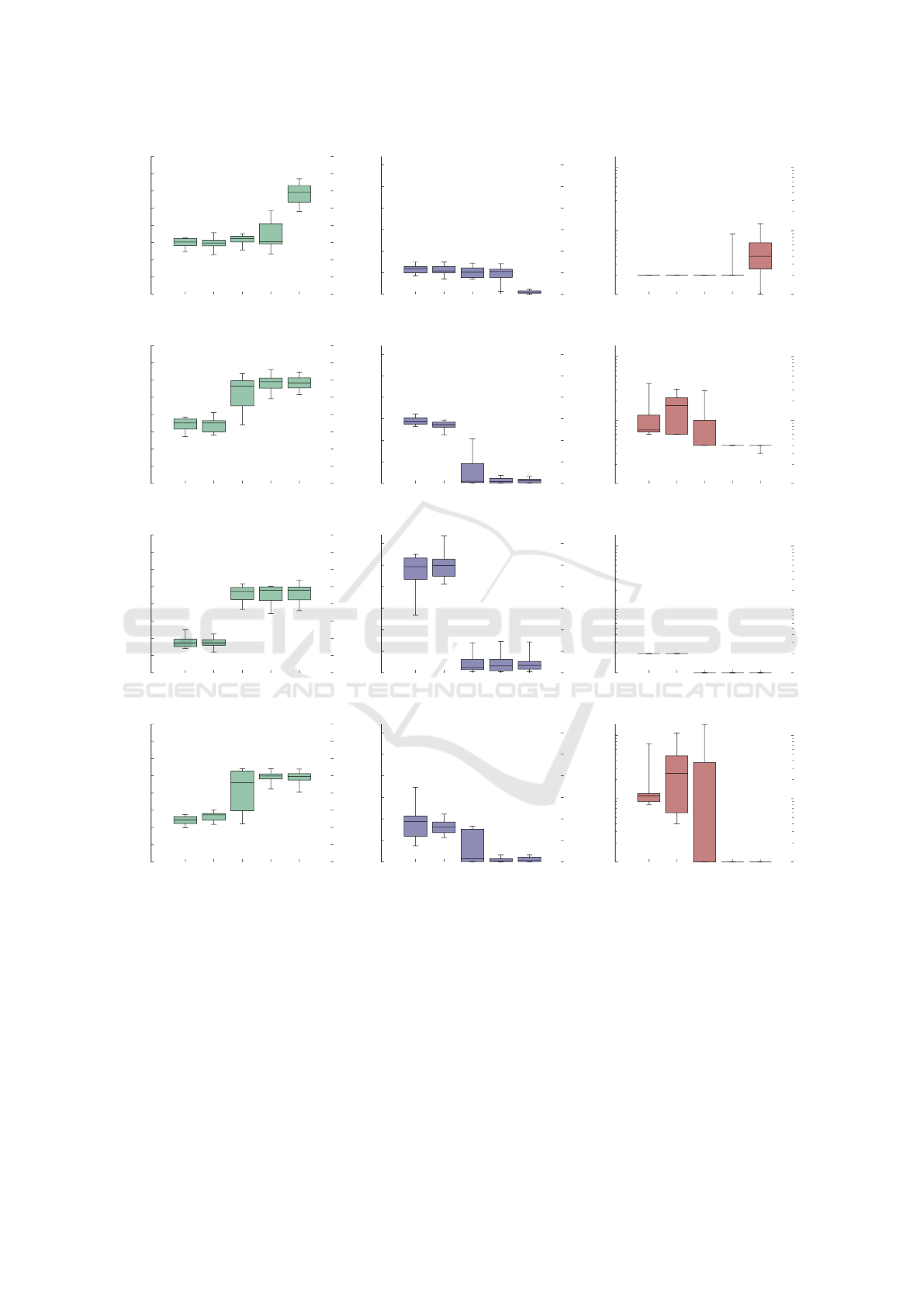
The NRMSE, storage ratio and number of iterations
required to reach the stopping criterion, averaged over
the datasets, are shown in Figure 2. Each boxplot
shows the interquartile and median error values for
NRMSE and storage metrics of the best reduction for
each dataset. The whiskers on each boxplot show the
minimum and maximum reported of all results.
We can draw several conclusions regarding the ap-
plication of 2D-STR to the datasets considered in this
paper. First, more accurate summaries of the dataset
occurred when α was small (e.g. α ∈ {0.01,0.1})
and model accuracy was favoured over storage vol-
ume. Conversely the opposite was true when α was
large (e.g. α ∈ {1,2}). Second, DCT summaries
(DCT-R and DCT-C) tended to yield more accurate
summaries than polynomial regression (PLR-R and
PLR-C) given the same α parameter value. Third,
values for α in the middle of the range of those evalu-
ated tended to give less consistent results, as indicated
by the larger interquartile range and extreme values
shown. Finally, the lower NRMSE values reported
for modelling on regions (PLR-R and DCT-R) shows
that modelling on regions yielded slightly more accu-
rate representations than modelling on clusters.
As shown in Figure 2, summary modelling on
regions (PLR-R and DCT-R) required significantly
fewer iterations to reach the stop criterion. Mod-
elling on clusters (PLR-C and DCT-C) required sig-
nificantly more iterations, and the modelling process
took longer owing to the larger number of instances
within each model. It was noted that modelling on re-
gions yielded fewer regions for lower α values than
modelling on clusters because the latter method re-
sults in fewer models which in turn have a higher error
when compared to their instances. Polynomial regres-
sion modelling (PLR-R and PLR-C) resulted in many
models when α was small, each of which was simple,
and few models when α was large, all of which were
more complex. Discrete cosine modelling (DCT-R
and DCT-C) was found to behave similarly when α
was small, whilst at larger α values the best iteration
was often the first, with one DCT coefficient stored
for the entire dataset. For large values of α, neither
increasing the number of regions nor increasing the
complexity of the existing DCT model gave a lower
storage ratio (q(D,(R,M))) than the first step. This re-
sult may help to explain why such models gave worse
NRMSE scores but yielded very low storage values.
Overall, these results show that it is possible to
reduce a spatio-temporal traffic sensor dataset signif-
icantly whilst incurring tolerable errors. In different
scenarios, different choices of α and modelling tech-
nique may be desirable. When model accuracy is im-
portant, DCT modelling on either regions or clusters
(DCT-R or DCT-C) may be preferable. These meth-
ods gave between 2.4% and 5.5% NRMSE when α
was 0.01 and 0.1. When modelling on clusters (DCT-
C) with α = 0.1, less than 12% of the original data
volume was required to reach these error rates. Whilst
higher NRMSE values indicate that the modelling
does not fit the instances so well, the smooth regres-
sions output captures the low-frequency trends of the
dataset well and removes some of the high-frequency
fluctuations in the dataset. This smoothing effect can
be used as a way of reducing noise in the dataset.
When few output models are desired, modelling
on clusters (PLR-C and DCT-C) is useful. Polynomial
regression modelling on clusters (PLR-C) yielded a
maximum of 7 models per feature for the entire re-
duced dataset and DCT modelling (DCT-C) yielded a
maximum of 12 models per feature. This may be par-
ticularly useful for applications where interpretation
of the output models is desired.
A low number of regions can be found by us-
ing high α values across all of the modelling tech-
niques evaluated. In particular, DCT modelling on
regions (DCT-R) consistently yielded a low number
of regions for α = 0.5,1.0 and 2.0 whilst the aver-
age NRMSE error was less than 10%. Again, this
GISTAM 2019 - 5th International Conference on Geographical Information Systems Theory, Applications and Management
48
0
2
4
6
8
10
12
14
16
0.01 0.1 0.5 1.0 2.0
AverageNRMSEoverallfeatures(%error)
Valueofalphaparameter
(a) NRMSE for PLR-R
0
5
10
15
20
25
30
0.01 0.1 0.5 1.0 2.0
Storageofreduceddataset(%oforiginalvolume)
Valueofalphaparameter
(b) Storage ratio for PLR-R
1
10
100
0.01 0.1 0.5 1.0 2.0
Numberofiterationstomeetoptimalreduction
Valueofalphaparameter
(c) Number of iterations for PLR-R
0
2
4
6
8
10
12
14
16
0.01 0.1 0.5 1.0 2.0
AverageNRMSEoverallfeatures(%error)
Valueofalphaparameter
(d) NRMSE for PLR-C
0
5
10
15
20
25
30
0.01 0.1 0.5 1.0 2.0
Storageofreduceddataset(%oforiginalvolume)
Valueofalphaparameter
(e) Storage ratio for PLR-C
1
10
100
0.01 0.1 0.5 1.0 2.0
Numberofiterationstomeetoptimalreduction
Valueofalphaparameter
(f) Number of iterations for PLR-C
0
2
4
6
8
10
12
14
16
0.01 0.1 0.5 1.0 2.0
AverageNRMSEoverallfeatures(%error)
Valueofalphaparameter
(g) NRMSE for DCT-R
0
5
10
15
20
25
30
0.01 0.1 0.5 1.0 2.0
Storageofreduceddataset(%oforiginalvolume)
Valueofalphaparameter
(h) Storage ratio for DCT-R
1
10
100
0.01 0.1 0.5 1.0 2.0
Numberofiterationstomeetoptimalreduction
Valueofalphaparameter
(i) Number of iterations for DCT-R
0
2
4
6
8
10
12
14
16
0.01 0.1 0.5 1.0 2.0
AverageNRMSEoverallfeatures(%error)
Valueofalphaparameter
(j) NRMSE for DCT-C
0
5
10
15
20
25
30
0.01 0.1 0.5 1.0 2.0
Storageofreduceddataset(%oforiginalvolume)
Valueofalphaparameter
(k) Storage ratio for DCT-C
1
10
100
0.01 0.1 0.5 1.0 2.0
Numberofiterationstomeetoptimalreduction
Valueofalphaparameter
(l) Number of iterations for DCT-C
Figure 2: Reduction results over traffic sensor datasets. Each sub-figure shows the results from 2D-STR using 5 values for
the parameter α, which weights model accuracy against storage ratio. The left column reports NRMSE averaged across the
features in the datasets. The middle column reports the quantity of data output by the reduction as a percentage of the original
data volume. The right column reports the number of iterations used by the algorithm. Results are shown for polynomial
regression on each region (PLR-R), polynomial regression on each cluster (PLR-C), discrete cosine modelling on each region
(DCT-R) and discrete cosine modelling on each cluster (DCT-C).
would be particularly useful for interpretability, in-
cluding fast visualisation of the whole dataset.
Finally, when a fast reduction is required, poly-
nomial and DCT modelling on regions (PLR-R and
DCT-R) is useful, particularly when α = 0.01 or 0.1.
These results showed small NRMSE error rates com-
pared to other techniques and parameter settings eval-
uated, whilst requiring significantly fewer iterations.
As expected, the α parameter was shown to trade
summary model accuracy for volume reduction at a
2D-STR: Reducing Spatio-temporal Traffic Datasets by Partitioning and Modelling
49

predictable rate. When α = 0.5 we observed higher
variance in each of the metrics used, indicating mixed
results may be seen for this setting. We suggest that
α = 0.5 is specific to traffic data and may be different
for other types of spatio-temporal data.
6.3 Comparison with Other Techniques
For the datasets considered in this paper, IDEALEM
gave a high reduction in the data volume, achieving
an average NRMSE of 3.6% for A roads and 4.4%
for motorways. This reduction performed poorly
in error, however, with an average storage ratio of
47.4% achieved across all features for A roads and
52.1% NRMSE across all features for motorways.
These large NRMSE values may be attributed to the
diverse temporal patterns exhibited within the files.
Since IDEALEM replaces statistically similar tempo-
ral blocks with references to the first occurrence of a
similar block, it fails to capture the nuances of traffic
patterns that vary across different time periods.
A plot of storage ratio against NRMSE for IDE-
ALEM can be seen in Figure 3. Similar NRMSE val-
ues and storage ratios were achieved for datasets sam-
pled from the same road regardless of the time period.
As seen above, IDEALEM performed better on most
A roads compared to motorways, achieving lower
NRMSE and storage ratios. Conversely, NRMSE and
storage ratios were more varied for samples taken at
the same time from different roads. This implies that
the spatial nature of the data has a stronger influ-
ence on the storage ratio and NRMSE than the tem-
poral nature, when using IDEALEM. Furthermore, it
may indicate that, whilst the raw values of instances
may change from month to month, the traffic pat-
terns of each road remain the same across the different
monthly observations in the datasets.
Results for DEFLATE show similar groupings as
IDEALEM. Whilst the NRMSE for DEFLATE is al-
ways 0, since DEFLATE is a lossless compression
method, A roads tend to result in lower storage ratios
than motorways. DEFLATE compressed data from A
roads to 17.4% of their original data volume on av-
erage, whereas data from motorways were reduced to
18.9%. This higher value for motorways may be in-
dicative of a higher variance in the motorway data.
Similar to IDEALEM, DEFLATE also shows that in-
dividual roads exhibit more similar compression ra-
tios across different time periods than data taken from
different roads during the same time period.
Several observations can be made regarding the
results for PCA. First, like DEFLATE and IDE-
ALEM, the temporal window used for sampling has
little effect on the resulting NRMSE. Second, the road
0
5
10
15
20
0 10 20 30 40 50 60 70 80
AverageNRMSEoverallfeatures(%error)
StorageRatio(%)
PCA 1 ComponentPCA 1 ComponentPCA 1 ComponentPCA 1 ComponentPCA 1 ComponentPCA 1 Component
PCA 4 ComponentsPCA 4 ComponentsPCA 4 ComponentsPCA 4 ComponentsPCA 4 ComponentsPCA 4 Components
DEFLATEDEFLATEDEFLATEDEFLATEDEFLATEDEFLATE
IDEALEMIDEALEMIDEALEMIDEALEMIDEALEMIDEALEM
2D-STR (PLR-R, α=0.1)2D-STR (PLR-R, α=0.1)2D-STR (PLR-R, α=0.1)2D-STR (PLR-R, α=0.1)2D-STR (PLR-R, α=0.1)2D-STR (PLR-R, α=0.1)
2D-STR (DCT-C, α=1.0)2D-STR (DCT-C, α=1.0)2D-STR (DCT-C, α=1.0)2D-STR (DCT-C, α=1.0)2D-STR (DCT-C, α=1.0)2D-STR (DCT-C, α=1.0)
Figure 3: Comparison of storage ratio and NRMSE in-
troduced by IDEALEM, PCA (1 and 4 components), DE-
FLATE, 2D-STR using polynomial regression on regions
(PLR-R) when α = 1.0 and 2D-STR using discrete cosine
modelling on clusters (DCT-C) when α = 1.0. These mod-
elling methods and parameter values were chosen to repre-
sent the range of results observed. Results for data sampled
from motorways are shown in blue and data sampled from
A roads shown in red.
location has some effect on the error rate, with dif-
ferent time periods taken from the same road achiev-
ing similar error rates across all numbers of principle
components (PCs). Using a single PC, PCA achieved
a 6.3% error on A roads and 8.2% on motorways,
whilst it achieved 1.2% and 1.8% error respectively
when using 4 components. In achieving these error
rates, PCA used 37.5% of the original data volume to
store a single PC and 75% to store 4 PCs. Finally, as
the number of components increased the error rate de-
creased significantly. When more than 5 components
were chosen the error rate was 0 or negligible across
all features and datasets. Furthermore, the spread of
error rates also decreased as the number of compo-
nents increased.
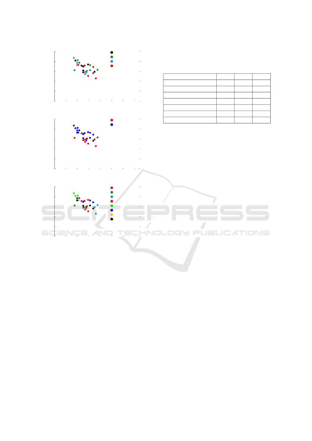
Figure 4 shows the NRMSE and storage used by
2D-STR when using polynomial regression on each
region (PLR-R) with α = 0.1. The class of road is
shown to impact the reduction achieved, as observed
with the previous techniques. Again, results were
clustered more by the road than time period, and simi-
lar results were observed for all modelling techniques
considered, except polynomial regression on regions
when α = 1.0 or 2.0. These results indicate that 2D-
STR is capable of achieving NRMSE rates similar
to those achieved by IDEALEM on 2-dimensional
spatio-temporal data. It is capable of achieving simi-
lar rates to PCA when a small number of components
is chosen, whilst achieving smaller storage ratios than
both PCA and IDEALEM.
Finally, a comparison of the time taken to re-
duce the datasets is shown in Table 3. These re-
sults indicate that whilst 2D-STR is capable of reduc-
ing 2-dimensional spatio-temporal data to a smaller
GISTAM 2019 - 5th International Conference on Geographical Information Systems Theory, Applications and Management
50
0
2
4
6
8
10
0 2 4 6 8 10 12 14
AverageNRMSEoverallfeatures(%error)
StorageRatio(%)
Apr '17
Sept '17
Nov '17
Dec '17
(a) Coloured by month
0
2
4
6
8
10
0 2 4 6 8 10 12 14
AverageNRMSEoverallfeatures(%error)
StorageRatio(%)
A Road
Motorway
(b) Coloured by road class
0
2
4
6
8
10
0 2 4 6 8 10 12 14
AverageNRMSEoverallfeatures(%error)
StorageRatio(%)
A30
A66
A69
M11
M1
M20
M23
M56
(c) Coloured by road
Figure 4: Comparison of storage ratio and NRMSE intro-
duced by 2D-STR using polynomial regression on each re-
gion (PLR-R) with α = 0.1. Here, (a) presents the results
of these reductions coloured by the month the dataset was
sampled from, (b) presents the results coloured by the type
of road, and (c) presents the results coloured by the road the
samples were taken from.
data volume than established methods, and achieves a
smaller NRMSE in doing so, the computation time
is much greater. This suggests that existing meth-
ods may be more useful when a faster reduction is
required. However, 2D-STR is more effective when
longer running times are permitted for reduction. It is
important to note that the implementation of 2D-STR
may be optimised further, and the running time of the
algorithm reduced as a result.
Table 3: Running time (wall time, in minutes) of the algo-
rithms presented in Section 6, over all of the datasets intro-
duced in Section 5. Results are shown for 2D-STR when
α ∈ {0.01,0.1, 0.5,1.0,2.0}.
Min Avg Max
2D-STR using PLR-R <1 545 3,699
2D-STR using PLR-C 14 26 38
2D-STR using DCT-R 18.7 249 1,870
2D-STR using DCT-C 2,542 3,457 3,711
IDEALEM <1 <1 <1
DEFLATE <1 <1 <1
PCA <1 <1 <1
7 CONCLUSION
In this paper, we proposed a novel method, 2D-STR,
for reducing spatio-temporal traffic datasets by ex-
ploiting regions of similar instances. The effective-
ness of 2D-STR has been demonstrated, in achiev-
ing a 96.3% reduction of the traffic sensor data whilst
only introducing a small error (< 3.7%), sufficiently
low to make the resulting data useful for many traffic
analysis tasks. We demonstrated 2D-STR on medium
sized traffic datasets but we believe it could scale to
much larger datasets and enable faster processing for
queries and analysis. In comparison to other tech-
niques, 2D-STR is found to reduce the dataset to sizes
similar to the DEFLATE method whilst achieving
NRMSE error rates similar to IDEALEM and PCA.
2D-STR is therefore shown to perform comparably to
commonly used techniques whilst enabling a wider
range of queries to be answered on the reduced data.
Working with reduced datasets makes analysis
possible on modest hardware that would otherwise
require greater computational resources. The inter-
polation nature of the modelling we have adopted in
this paper permits many applications, such as spatio-
temporal data linkage. Future extensions of this work
could investigate reduction over the entire road net-
work, larger datasets, and other modelling techniques.
Furthermore, extensions of the technique for other
types of data should be explored.
ACKNOWLEDGEMENTS
The lead author gratefully acknowledges funding by
the UK Engineering and Physical Sciences Research
Council (grant no. EP/L016400/1), the EPSRC Cen-
tre for Doctoral Training in Urban Science. The lead
author also gratefully acknowledges funding by TRL.
2D-STR: Reducing Spatio-temporal Traffic Datasets by Partitioning and Modelling
51

REFERENCES
Acampora, G., Tortora, G., and Vitiello, A. (2016). Com-
parison of Multi-objective Evolutionary Algorithms
for prototype selection in nearest neighbor classifica-
tion. In SSCI 2016, pages 1–8.
Berberidis, D. and Giannakis, G. B. (2015). Data sketch-
ing for tracking large-scale dynamical processes. In
ACSSC 2015, pages 345–349.
Berberidis, D. and Giannakis, G. B. (2017). Data Sketching
for Large-Scale Kalman Filtering. IEEE Transactions
on Signal Processing, 65(14):3688–3701.
Birvinskas, D., Jusas, V., Martisius, I., and Damasevicius,
R. (2012). EEG Dataset Reduction and Feature Ex-
traction Using Discrete Cosine Transform. In 2012
Sixth UKSim/AMSS European Symposium on Com-
puter Modeling and Simulation, pages 199–204.
Bloom, B. H. (1970). Space/Time Trade-offs in Hash
Coding with Allowable Errors. Commun. ACM,
13(7):422–426.
Cormode, G., Garofalakis, M., Haas, P. J., and Jermaine,
C. (2012). Synopses for massive data: Samples, his-
tograms, wavelets, sketches. Foundations and Trends
in Databases, 4(1–3):1–294.
Cormode, G. and Muthukrishnan, S. (2005). An improved
data stream summary: the count-min sketch and its
applications. Journal of Algorithms, 55(1):58–75.
Deutsch, P. (1996). Deflate compressed data format speci-
fication version 1.3. Technical report.
Fahad, A., Alshatri, N., Tari, Z., Alamri, A., Khalil, I.,
Zomaya, A. Y., Foufou, S., and Bouras, A. (2014). A
Survey of Clustering Algorithms for Big Data: Tax-
onomy and Empirical Analysis. IEEE Transactions
on Emerging Topics in Computing, 2(3):267–279.
Flajolet, P., Fusy,
´
E., Gandouet, O., and Meunier, F. (2007).
Hyperloglog: the analysis of a near-optimal cardinal-
ity estimation algorithm. In Discrete Mathematics and
Theoretical Computer Science, pages 137–156.
Garcia, S., Derrac, J., Cano, J., and Herrera, F. (2012).
Prototype Selection for Nearest Neighbor Classifica-
tion: Taxonomy and Empirical Study. IEEE Trans-
actions on pattern analysis and machine intelligence,
34(3):417–435.
Guo, T., Yan, Z., and Aberer, K. (2012). An Adaptive Ap-
proach for Online Segmentation of Multi-dimensional
Mobile Data. In Proceedings of the Eleventh ACM In-
ternational Workshop on Data Engineering for Wire-
less and Mobile Access, pages 7–14. ACM.
Lakshminarasimhan, S., Jenkins, J., Arkatkar, I., Gong, Z.,
Kolla, H., Ku, S. H., Ethier, S., Chen, J., Chang, C. S.,
Klasky, S., Latham, R., Ross, R., and Samatova, N. F.
(2011). ISABELA-QA: Query-driven analytics with
ISABELA-compressed extreme-scale scientific data.
In SC 2011, pages 1–11.
Lemley, J., Jagodzinski, F., and Andonie, R. (2016). Big
Holes in Big Data: A Monte Carlo Algorithm for De-
tecting Large Hyper-Rectangles in High Dimensional
Data. In COMPSAC 2016, pages 563–571.
Li, J., Cheng, K., Wang, S., Morstatter, F., Trevino, R. P.,
Tang, J., and Liu, H. (2017). Feature Selection: A
Data Perspective. ACM Comput. Surv., 50(6):94:1–
94:45.
Martinez, A. M. and Kak, A. C. (2001). PCA versus LDA.
IEEE Transactions on pattern analysis and machine
intelligence, 23(2):228–233.
Mukahar, N. and Rosdi, B. A. (2018). Performance com-
parison of prototype selection based on edition search
for nearest neighbor classification. In Proceedings
of the 2018 7th International Conference on Software
and Computer Applications, ICSCA 2018, pages 143–
146. ACM.
Ougiaroglou, S. and Evangelidis, G. (2012). Efficient
Dataset Size Reduction by Finding Homogeneous
Clusters. In Proceedings of the Fifth Balkan Confer-
ence in Informatics, pages 168–173. ACM.
Pan, B., Demiryurek, U., Banaei-Kashani, F., and Sha-
habi, C. (2010). Spatiotemporal Summarization of
Traffic Data Streams. In Proceedings of the ACM
SIGSPATIAL International Workshop on GeoStream-
ing, pages 4–10. ACM.
Pearson, K. (1901). LIII. On lines and planes of closest fit to
systems of points in space. The London, Edinburgh,
and Dublin Philosophical Magazine and Journal of
Science, 2(11):559–572.
Roweis, S. T. and Saul, L. K. (2000). Nonlinear dimension-
ality reduction by locally linear embedding. science,
290(5500):2323–2326.
Samet, H. (1984). The quadtree and related hierarchical
data structures. ACM Comput. Surv., 16(2):187–260.
Sisovic, S., Bakaric, M. B., and Matetic, M. (2018). Re-
ducing Data Stream Complexity by Applying Count-
Min Algorithm and Discretization Procedure. In 2018
IEEE Fourth International Conference on Big Data
Computing Service and Applications (BigDataSer-
vice), pages 221–228.
Tai, K. S., Sharan, V., Bailis, P., and Valiant, G. (2018).
Sketching Linear Classifiers over Data Streams. In
Proceedings of the 2018 International Conference on
Management of Data, pages 757–772. ACM.
Tenenbaum, J. B., De Silva, V., and Langford, J. C. (2000).
A global geometric framework for nonlinear dimen-
sionality reduction. science, 290(5500):2319–2323.
Wang, M., Li, H. X., and Shen, W. (2016). Deep auto-
encoder in model reduction of lage-scale spatiotempo-
ral dynamics. In 2016 International Joint Conference
on Neural Networks (IJCNN), pages 3180–3186.
Wong, L. Z., Chen, H., Lin, S., and Chen, D. C. (2014).
Imputing Missing Values in Sensor Networks Us-
ing Sparse Data Representations. In Proceedings of
the 17th ACM International Conference on Modeling,
Analysis and Simulation of Wireless and Mobile Sys-
tems, pages 227–230. ACM.
Wu, K., Lee, D., Sim, A., and Choi, J. (2017). Statistical
data reduction for streaming data. In 2017 New York
Scientific Data Summit (NYSDS), pages 1–6.
Xue, B., Zhang, M., Browne, W. N., and Yao, X. (2016). A
Survey on Evolutionary Computation Approaches to
Feature Selection. IEEE Transactions on Evolution-
ary Computation, 20(4):606–626.
GISTAM 2019 - 5th International Conference on Geographical Information Systems Theory, Applications and Management
52
