
Accelerated RRT* and Its Evaluation on Autonomous Parking
Jiri Vlasak
12
, Michal Sojka
2
and Zdenˇek Hanz´alek
2
1
Faculty of Electrical Engineering, Czech Technical University in Prague, Technicka 2, Prague, Czech Republic
2
Czech Institute of Informatics, Robotics and Cybernetics, Czech Technical University in Prague,
Jugoslavskych partyzanu 1580/3, Prague, Czech Republic
Keywords:
Autonomous Parking, Rapidly-Exploring Random Trees, Reeds and Shepp Steering, Dijkstra Optimization,
Nearest Neighbor Heuristics.
Abstract:
Finding a collision-free path for autonomous parking is usually performed by computing geometric equations,
but the geometric approach may become unusable under challenging situations where space is highly con-
strained. We propose an algorithm based on Rapidly-Exploring Random Trees Star (RRT*), which works
even in highly constrained environments and improvements to RRT*-based algorithm that accelerate compu-
tational time and decrease the final path cost. Our improved RRT* algorithm found a path for parallel parking
maneuver in 95 % of cases in less than 0.15 seconds.
1 INTRODUCTION
Modern cars are commonly equipped with parking
assistants that can perform parallel or perpendicular
parking maneuvers. Parking is a relatively easy task
as the movement is slow and the car dynamics might
be neglected. Usually, geometric equations are used
for planning these maneuvers. A geometric approach
has limitations when applied in unexpected environ-
ments or when more than a simple parking maneuver
has to be planned. In this paper we address the cases,
when more advanced planners need to be used, and
one of the problems experienced by those complex
planners is their computational complexity.
For this paper, we define the parking problem as
finding a collision-free path from an initial car posi-
tion (i.e., x, y, and heading) to the goal position under
the presence of an arbitrary number of known static
obstacles. The path may consist of an arbitrary num-
ber of path segments alternating forward and back-
ward drives of the car. We are interested in a close
to optimal parking maneuver path in the sense of path
length respecting the kinematic constraints of the car.
In this paper, we propose an RRT*-based al-
gorithm to solve the autonomous parking problem,
which we define more formally in Section 2. Con-
trary to well-known A* algorithm, RRT* algorithm
does not need space discretization. Also, it handles
nonholonomic constraints by design. The RRT* al-
gorithm searches the state space by creating a tree
structure that represents possible paths. RRT*-based
algorithms were successfully applied to a wide range
of planning problems from the robot, vehicle, and
aerial domains. However, they were also used in not
such apparentproblemsas tunnel detection in proteins
from the field of molecular biology.
Our algorithm uses Reeds and Shepp curves for
particular path segments when building the tree and
Euclidean distance as a metric for the nearest neigh-
bor search. We complemented the RRT* algorithm
with an optimization procedure based on the Dijkstra
algorithm used to reduce the number of the path seg-
ments and to lower the cost of the path connecting
initial and goal pose.
The main contributions of this paper are:
• Minimization of the path cost with an optimiza-
tion procedure based on the shortest path by Dijk-
stra algorithm.
• Speed up of the RRT* path search with the nearest
neighbor heuristics.
In our experiments (see Section 5), we compare
multiple cost functions of the nearest neighbor search
and show that the fastest approach to find the path is
to use the Euclidean distance as the cost function in
the nearest neighbor search (see Figure 4). We also
evaluate the effectiveness of our optimization proce-
dure based on the Dijkstra algorithm and show (see
Figure 5) that it significantly improves the cost of the
path even when compared to other algorithms such as
86
Vlasak, J., Sojka, M. and Hanzálek, Z.
Accelerated RRT* and Its Evaluation on Autonomous Parking.
DOI: 10.5220/0007679500860094
In Proceedings of the 5th International Conference on Vehicle Technology and Intelligent Transport Systems (VEHITS 2019), pages 86-94
ISBN: 978-989-758-374-2
Copyright
c
2019 by SCITEPRESS – Science and Technology Publications, Lda. All rights reserved
RRT*-Smart. In Section 6 we summarize our results.
The source code of our algorithm is available
1
.
1.1 Related Works
A common approach to solve a parking problem is to
split the task to the environment detection, the path
planning, and the path execution. In this paper, we
consider the path planning part.
Typical parking problems can be classified into
two classes: parallel parking and perpendicular park-
ing. Some publications consider only parallel parking
(Gupta et al., 2010), (Cheng et al., 2013), (Vorobieva
et al., 2013), or only perpendicular parking (Petrov
et al., 2015). In this paper, we propose a universal
method which considers obstacles of arbitrary shape.
Many published approaches use Reeds and Shepp
curves (Reeds and Shepp, 1990) for path plan-
ning (Lee et al., 2006) without considering obsta-
cles. In (Fraichard and Scheuer, 2004), the authors
present Continuous-Curvature Paths that extend the
Reeds and Shepp line segments and circular arcs with
clothoid arcs. Resulting paths have continuous cur-
vature, so a car that follows a path does not have to
stop to change orientation of the wheels. Continuous-
Curvature Paths have been used in (Muller et al.,
2007), (Vorobieva et al., 2013), (Cheng et al., 2013),
and (Yi et al., 2017). In (Kim et al., 2010), the au-
thors use two basic motions to create a set of motions.
Finally, (Hsu et al., 2008), (Gupta et al., 2010), and
(Liang et al., 2012) describe parking using paths gen-
erated with two circles geometry.
However, in real-life situations, a typical parking
scenario may be disturbed by sloppy parked neigh-
bor car, temporary parked bike, non-standard parking
slot shape, or other unspecified constraints. There-
fore, when a parking slot is detected, evaluation of a
situation may fail, and an approach based on geomet-
ric equations may become unusable in such a case.
In this paper, we propose RRT*-based algo-
rithm which can handle complex parking situations.
Rapidly-Exploring Random Trees (RRT) (LaValle,
1998) is a randomized algorithm that can handle non-
holonomic constraints. Although RRT is probabilisti-
cally complete (with probability 1, the algorithm con-
verges to the solution, as time tends to infinity), it
is not asymptotically optimal (Karaman and Frazzoli,
2011). Therefore, Karaman and Frazzoli proposed the
RRT* algorithm, which converges to an optimal solu-
tion as time tends to infinity. In (Islam et al., 2012),
the authors improved the RRT* algorithm by using
path optimization and intelligent sampling and named
the resulting algorithm RRT*-Smart. After the initial
1
http://rtime.felk.cvut.cz/gitweb/hubacji1/iamcar.git
path is found, RRT*-Smart converges to the optimum
faster than RRT*. In our approach, we stop the RRT*
algorithm when a path is found, and then we optimize
the path by Dijkstra algorithm.
2 THE PARKING PROBLEM
In this section, we define the problem and terminol-
ogy used throughout this paper.
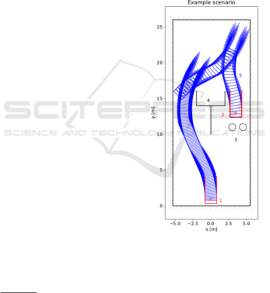
Figure 1: Example scenario with the init pose (1), the goal
pose (2), two circle obstacles (3), the obstacle compound of
line segment obstacles (4), and the final path (5).
A pose is a triplet p = (x, y, θ), where x, y are carte-
sian coordinates and θ is a heading.
A search space is a set of poses S = {(x, y, θ) | x ∈
[XMIN, XMAX],y ∈ [YMIN,YMAX],θ ∈ [0, 2π)},
where XMIN, XMAX,YMIN, andYMAX are borders
of search space.
Accelerated RRT* and Its Evaluation on Autonomous Parking
87

A scenario is a quintuple s =
(S, p
init
, p
goal
, O
C
, O
S
), where S is a search space,
p
init
, p
goal
are init and goal poses, and O
C
resp.
O
S
are sets of circle obstacles resp. line segment
obstacles. We can see an example scenario with
the final path connecting initial and goal pose in
Figure 1. Example scenario also demonstrates
segment obstacles (borders), circle obstacles, and the
complex obstacle of arbitrary shape (compound of
line segment obstacles).
Circle obstacle is a triplet o
c
= (x, y, r), where
x, y are cartesian coordinates of the center, and r is
the radius. Line segment obstacle is a quadruple
o
s
= (x
1
, y
1
, x
2
, y
2
), where x
1
, y
2
are coordinates of the
line segment start and x
2
, y
2
are coordinates of the line
segment end.
A car is a quadruple c = (l, w,R, b), where l is a
length of the car, w is a width of the car, R =
1
κ
is car
minimum turning radius, κ is curvature, and b is car
wheelbase (the distance between front and rear axles).
In Figure 1, red crosses represent x, y coordinates of
init and goal poses. The U-Shape frame represents
length l, width w, and pose heading. Finally, example
obstacles are hatched.
A path from pose a to pose b is a sequence of
poses P
a,b
= {p
i
| i ∈ {0, 1, ...,n − 1}, p
0
= a, p
n−1
=
b}, such that P satisfies kinematic constrains given by
car c.
The collide(p, O) function returns True when a
car c positioned at pose p is inside arbitrary obstacle
o ∈ O, or the frame of car c collides with this obstacle.
Otherwise, the function returns False.
The collide(P, O) function returns True when for
any pose p ∈ P the collide(p, O) returns True. Oth-
erwise, the function returns False.
The cost(P) is a path cost defined in Equation 1,
where RSDist(a, b) is Reeds & Shepp distance from
pose a to pose b.
cost(P) =
i=n−2
∑
i=0
RSDist(p
i
, p
i+1
) (1)
We define final path P
F
in Equation 2, where
P
all
= {P
a,b
| a = p
init
, b = p
goal
, ¬collide(P, O)}. An
example of the final path is in Figure 1.
P
F
= argmin
P
P∈P
all
cost(P) (2)
3 RRT*
Rapidly-Exploring Random Tree Star (RRT*) is
an asymptotically optimal randomized algorithm to
solve path planning problems, such as the parking
problem defined in Section 2.
RRT* uses a tree data structure that represents
poses and paths, it handles nonholonomic constraints
and can hold general restrictions on p
init
and p
goal
poses, or obstacles. Therefore, the RRT* should be
able to solve the unpredictable, real-life scenarios. We
can see basic RRT* pseudocode (lines 4 to 19) as part
of complete RRT*-based Algorithm 1.
The fundamental element of RRT* is a node. The
node is a poseextended with parent (the pointer to the
predecessor node), children (the array of successor
nodes), and cumulative cost ccost = cost(P
p
init
,node
).
As node is extension to pose, we may update our def-
inition of path P
a,b
= {p
i
| i ∈ {0, 1, ..., n − 1}, p
0
=
a, p
n−1
= b}, such that a, b, and p
i
are nodes, where
p
i
is parent of p
i+1
. We use a path as the sequence of
poses or nodes interchangeably.
In RRT* algorithm, all nodes are stored in tree
data structure T = (root,V, E), where root node
corresponds to p
init
pose, V is set of nodes, E
is set of edges, and ∀n
1
, n
2
∈ V : {n
1
, n
2
} ∈ E ⇔
n
1
is the parent of n
2
.
3.1 Basic Procedures
In this section, we describe the basic procedures of
RRT* used to build T data structure.
RANDOMSAMPLE procedure returns a node with
a pose from search space S, where x, y, and θ are ran-
domly generated.
COST(nn, rs) function is a metric used in RRT*.
NEARESTNEIGHBOR(rs) procedure searches for
a node with the lowest COST(node,rs) in T .
STEER(nn, rs) procedure returns a path P
nn,rs
. We
can see the results of STEER procedure in Figure 2
(gray).
NEARNODES(ns, dist) procedure returns a set of
nodes nns from T , such that ∀n ∈ nns : COST(n, ns) <
dist.
CONNECT(ns, nns) procedure searches in near
nodes (nns) for the best candidate node to expand T
towards the ns. The best candidate node is the node
in T that minimizes the cumulative cost of ns when
it becomes the parent of the ns. The path from the
best candidate node to the ns must be free of col-
lisions. If the best candidate node is found, the na
is added as a child of the best candidate node, and
CONNECT(ns, nns) returns True. Otherwise, the pro-
cedure returns False.
REWIRE(ns, nns) procedure checks if for any
node in nns there is a path with lower cumulative cost
via ns. And swaps parents if so. This procedure along
VEHITS 2019 - 5th International Conference on Vehicle Technology and Intelligent Transport Systems
88
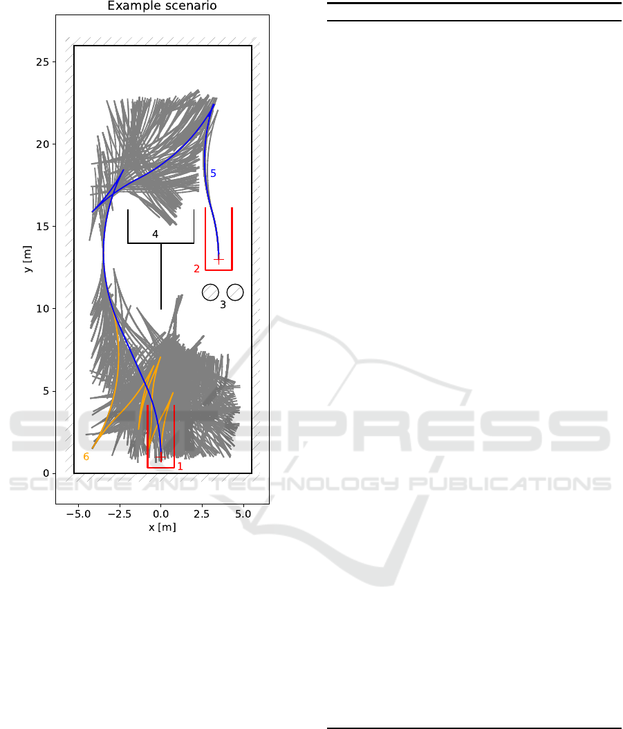
Figure 2: Example scenario with the init pose (1), the goal
pose (2), two circle obstacles (3), the obstacle compound
of line segment obstacles (4), the final path (5), the final
path before optimization (6), and line segments and circle
segments (gray).
with CONNECT(ns, nns) ensures the asymptotical op-
timality of RRT*.
GOALFOUND returns True if p
goal
∈ T and False
otherwise.
COLLIDES(na, ns) returns True if the path P
na,ns
collides with any obstacle of scenario, and False oth-
erwise.
3.2 Implementation
Our RANDOMSAMPLE procedure samples randomly
from the whole space S (including obstacles). We
use OMPL (Sucan et al., 2012) implementation of
Reeds and Shepp (Reeds and Shepp, 1990) optimal
paths for STEER and COST functions. NEARNODES,
Algorithm 1: Accelerated RRT*.
1: Input:
• initial pose
• goal pose
• array of obstacles
2: Output:
• True if goal pose reached, False otherwise
• array of paths connecting initial and goal pose
3: procedure RRT*
4: while ELAPSED < TMAX do
5: rs ← RANDOMSAMPLE
6: nn ← NEARESTNEIGHBOR(rs)
7: pn ← nn
8: newNodes ←
/
0
9: for ns ← STEER(nn, rs) do
10: nns ← pn∪ NEARNODES(ns, dist)
11: if CONNECT(ns, nns) then
12: REWIRE(ns, nns)
13: newNodes ← newNodes∪ ns
14: if GOALFOUND then
15: break while
16: end if
17: pn ← ns
18: end if
19: end for
20: for na ← newNodes do
21: pn ← na
22: for ns ← STEER(na, goal) do
23: if COLLIDE(pn, ns) then
24: break
25: end if
26: pn.children ← pn.children∪ ns
27: if GOALFOUND then
28: break while
29: end if
30: pn ← ns
31: end for
32: end for
33: end while
34: if GOALFOUND then
35: OPTPATH
36: end if
37: return GOALFOUND
38: end procedure
CONNECT and REWIRE procedures work the same as
in (Karaman and Frazzoli, 2011).
For two nodes we implemented auxiliary
ISNEAR(n
1
, n
2
) function that returns True if n
1
is within the predefined Euclidean distance from
n
2
(GFDIST) and the difference between head-
ings of n
1
and n
2
is less than the specified angle
(GFANGLE). We use this function to specify if the
Accelerated RRT* and Its Evaluation on Autonomous Parking
89

goal was found, the STEER procedure reached rs,
or if two nodes are the same. For computational
experiments in Section 5, we used GFDIST = 0.05
and GFANGLE =
π
32
.
In each iteration of RRT*-based algorithm, there
is an expansion of T towards the p
goal
(see lines 20
to 32 in Algorithm 1) as used in (Kuwata et al.,
2008). We added path optimization procedure to
RRT*-based algorithm (see line 35 in Algorithm 1)
that is run when the goal is found as explained in Sec-
tion 4.2. We can see an example of optimized final
path (5) and final path before optimization (6) in Fig-
ure 2.
4 RRT* IMPROVEMENTS
In this section, we introduce our improvementto near-
est neighbor search and details about path optimiza-
tion procedure.
4.1 Nearest Neighbor
Because the nearest neighbor procedure returns a
node with the lowest cost, such a node is a good candi-
date for tree expansion. The pseudocode of the near-
est neighbor search is outlined in Algorithm 2. To
improve the performance of finding the nearest neigh-
bor, we use a nodes data structure (the array of linked
lists of nodes) defined in line 3. The nodes data struc-
ture allows us to split search space S along the y-axis
(y− axis suits better for parallel parking scenario we
experimented with in Section 5), so we can compare
nodes within multiples of IYSTEP (increment dis-
tance based on nodes data structure) constant first.
Lines 7 to 10 describes how a node is added to
nodes. First, we compute the index of nodes array
(iy) where the node should be stored. Then, the node
is added to the list of nodes at that iy index.
When looking for the nearest neighborof the node
in the indexing structure (lines 14 to 30), we com-
pute iy index again. Then, we search the list of nodes
stored in the array nodes on index iy (nodes[iy]). Fi-
nally, we repeatedly widen the interval of indexes to
be investigated while the minimum cost is higher than
half of the interval width times IYSTEP and search
the lists of nodes stored in the array on indexes corre-
sponding to the widened interval.
We use Euclidean distance as the cost function in
the nearest neighbor search in contrast to Reeds and
Shepp path length as the cost function for building
RRT*. This approach speeds up the process but does
not influence the final path cost as discussed in Sec-
tion 5.
Algorithm 2: Nearest neighbor search.
1: IYSIZE ⊲ nn structure size
2: IYSTEP ⊲ increment distance
3: nodes[IYSIZE] ⊲ array of lists of nodes
4:
5: Input:
• node to be added to data structure
6: Output:
• data structure of nodes
7: procedure ADDIY(node)
8: iy ← ⌊
node.y
IYSTEP
⌋
9: nodes[iy] ← nodes[iy] ∪ node
10: end procedure
11:
12: Input:
• node to be searched
13: Output:
• the nearest neighbor of node
14: procedure NEARESTNEIGHBOR(node)
15: iy ← ⌊
node.y
IYSTEP
⌋
16: nn ← NULL ⊲ nearest neighbor
17: c
min
← ∞ ⊲ minimum cost
18: as ← 0 ⊲ array step
19: while c
min
> as· IYSTEP do
20: i ← max(iy− as, 0)
21: j ← min(iy+ as, IYSIZE − 1)
22: for n ∈ nodes[i] ∪ nodes[ j] do
23: if EDIST(n, node) < c
min
then
24: c
min
← EDIST(n, node)
25: nn ← n
26: end if
27: end for
28: as ← as+ 1
29: end while
30: end procedure
4.2 Path Optimization
The path optimization procedure is run when the goal
is found. Even that RRT* is asymptotically optimal, it
converges to the optimal solution very slowly. When
the p
goal
is reached for the first time a final path P
F
is probably far from optimum in the sense of cost (we
use Reeds and Shepp path length as cost). The pur-
pose of path optimization procedure is to decrease the
final path cost.
A final path P
F
consists of topologically ordered
nodes (see definition of a path in Section 2). We se-
lect tip nodes from the final path that are also topolog-
ically ordered. In our case, tip nodes are cusp nodes
(nodes where the direction of movement changes)
along with p
init
and p
goal
.
VEHITS 2019 - 5th International Conference on Vehicle Technology and Intelligent Transport Systems
90

Algorithm 3: Path optimization.
1: Input:
• path connecting initial and goal pose
2: Output:
• lowercost path connecting initial and goal pose
3: procedure OPTPATH
4: tips ← cusp nodes ⊲ array
5: pq ←
/
0 ⊲ priority queue
6: pq ← pq ∪ tips[0]
7: while |pq| 6= 0 do
8: n
i
← POP(pq)
9: if n
i
= tips[SIZE(tips) − 1] then
10: break
11: end if
12: for all j > i do
13: n
j
← tips[ j]
14: P
n
i
,n
j
← STEER(n
i
, n
j
)
15: c ← n
i
.ccost + COST(n
i
, n
j
)
16: if COLLIDE(n
i
, n
j
) then
17: continue
18: end if
19: if c < n
j
.ccost then
20: n
j
.ccost ← c
21: n
j
.parent ← i
22: if n
j
.visited = False then
23: n
j
.visited ← True
24: pq ← pq ∪ n
j
25: end if
26: end if
27: end for
28: end while
29: opath ←
/
0 ⊲ new optimized path
30: i ← SIZE(tips) − 1
31: while i > 0 do
32: opath ← opath∪tips[i]
33: i ← tips[i].parent
34: end while
35: opath ← opath∪ tips[0]
36: if better cost of opath then
37: return True
38: end if
39: return False
40: end procedure
In Algorithm 3 we initialize tip nodes and priority
queue in lines 4 to 6. In lines 7 to 28, we use Dijk-
stra algorithm to find the shortest path from the first
tip node (p
init
) to the last one (p
goal
). From the pri-
ority queue, we pop the node n
i
(where i is the index
of n
i
node in tips array) with the lowest cumulative
cost. Then, we call STEER(n
i
, n
j
) procedure from n
i
to all n
j
for j > i (see lines 12 to 27) that returns path
P
n
i
,n
j
. If P
n
i
,n
j
is collision free and cumulative cost of
n
j
is smaller when reached via P
n
i
,n
j
then parent and
cumulative cost of n
j
are updated, and n
j
is pushed to
the priority queue if not visited already. The process
repeats until the priority queue is empty or n
i
= p
goal
.
Optimized path found by Dijkstra is retrieved in
lines 29 to 35. If the cumulative cost of p
goal
is bet-
ter, OPTPATH procedure returns True and False oth-
erwise.
5 COMPUTATIONAL
EXPERIMENTS AND
EVALUATION
We present the results of computational experiments
for parallel parking scenario with no obstacle in Sec-
tion 5.1, and the results of computational experiments
for parallel parking scenarios with circle obstacle in
Section 5.2.
We are interested in the nearest neighbor search
and path optimization procedures. Specifically, we
are interested in how does the cost function, used
in the nearest neighbor search, influences algorithm
computation time. We experimented with the follow-
ing implementations of the nearest neighbor search:
• Nearest neighbor search with the cost based on
Reeds and Shepp path length.
• Nearest neighbor search with the cost based on
Reeds and Shepp path length but with the heading
of nodes temporarily set to the same value.
• Nearest neighbor search with the cost based on
Euclidean distance.
Also, we would like to know if the path optimiza-
tion procedure influences the cost of the final path.
We tested the following path optimization possibili-
ties:
• No path optimization.
• Path optimization from (Islam et al., 2012).
• Path optimization described in Algorithm 3.
The car we use for experiments is 1.625m wide
and 3.760m long. The minimum turning radius of
the car is 10.820 m and wheelbase is 2.450m.
We run computational experiments on a sin-
gle core of Intel(R) Core(TM) i7-5600U CPU @
2.60GHz with MemTotal: 16322516kB.
5.1 Scenario with No Obstacle
We tested RRT*-based algorithm on parallel parking
scenario shown in Figure 3. The parking lot is 2.2 m
Accelerated RRT* and Its Evaluation on Autonomous Parking
91
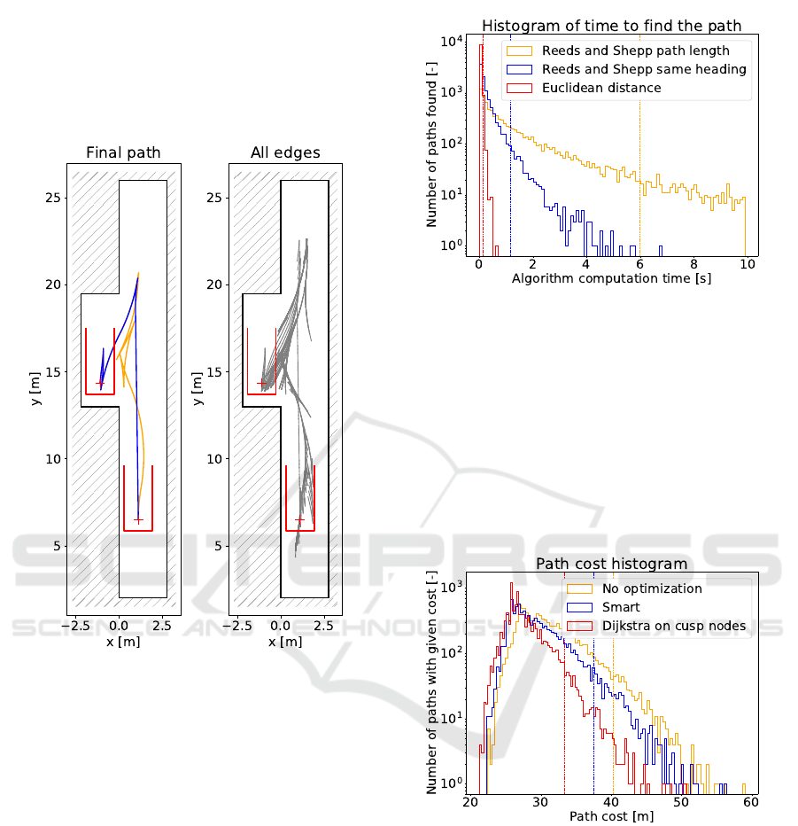
wide and 6.5 m long (CSN 73 6056, 2011). The width
of the street is 2.75m.
We let the Algorithm 1 to run for up to 10 seconds.
When the RRT*-based algorithm finds the goal, the
OPTPATH procedure optimizes the final path. We re-
peated the experiment 10000 times for this scenario.
Figure 3: Parallel parking scenario with no obstacle. On the
left, there is a final path before optimization (orange) and
optimized final path (blue). On the right, there is a complete
tree of all paths (gray).
5.1.1 Nearest Neighbor Search
We compare the computation times when the algo-
rithm found the final path for different cost functions
used in the nearest neighbor search implementations.
We can see the results in the histogram with the loga-
rithmic scale in Figure 4.
For the nearest neighbor search implementation
with the Reeds and Shepp cost function (the same cost
function used for building T , orange in Figure 4), the
algorithm did not find the goal in all runs. On the
other hand, for the nearest neighbor search implemen-
tation where we used the Euclidean distance as the
cost function (red in Figure 4), the goal was found in
100 % of runs. For comparison purposes, we run the
experiment for the nearest neighbor search implemen-
tation with Reeds and Shepp cost function, where the
heading of the nodes was temporarily set to the same
Figure 4: Histogram of time to find the path. Vertical
dashed lines represent 95 % percentile (red is 0.13, blue is
1.16, orange is 5.98).
value (blue in Figure 4).
5.1.2 Path Optimization
We also compared the final path costs for different
path optimization procedures. We can see the results
in the histogram with the logarithmic scale in Fig-
ure 5.
Figure 5: Path cost histogram. Vertical dashed lines repre-
sent 95 % percentile (red is 33.29, blue is 37.56, orange is
40.31).
We can see the improvement over no path opti-
mization (orange) when algorithm from (Islam et al.,
2012) is used (blue). And we can see that the path op-
timization from Algorithm 3 (red) has the best results.
5.2 Scenario with Circle Obstacle
Further, we tested RRT*-based algorithm on parallel
parking scenarios shown in Figure 6. The parking lot
is 2.2 m wide and 6.5m long (CSN 73 6056, 2011).
The width of the street is 2.75m. There is a random
VEHITS 2019 - 5th International Conference on Vehicle Technology and Intelligent Transport Systems
92

circle obstacle with diameter of 0.5 m laying on the
street near the parking lot.
We let the Algorithm 1 to run for up to 10 seconds.
When the RRT*-based algorithm finds the goal, the
OPTPATH procedure optimizes the final path. We re-
peated the experiment 10000 times for this scenario.
Figure 6: Parallel parking scenarios with circle obstacle.
Scenarios 1 and 2 differ in the position of circle obstacle.
There is the final path before optimization (orange) and the
optimized final path (blue).
The results are similar to the results in Section 5.1.
The cost based on the Euclidean distance speeds up
the algorithm computation time (95% percentile), de-
pendent on the obstacle position, to 0.12 s for Sce-
nario 1 and to 0.66s for Scenario 2. The path opti-
mization procedure decreases the cost of the final path
(95 % percentile) by 4% concerning No optimization
case for both scenarios.
6 CONCLUSION
We proposed the RRT*-based algorithm for plan-
ning parking paths and experimented with the nearest
neighbor search and path optimization procedures.
RRT*-based algorithm without improvements
uses the cost function based on the Reeds and Shepp
path length in the nearest neighbor search (as well as
for building the T data structure), and no optimiza-
tion procedure. Our improvements include the cost
function based on Euclidean distance in the nearest
neighbor search and optimization procedure based on
the Dijkstra algorithm.
We have shown that when we use the cost function
based on the Reeds and Shepp path length for build-
ing the T data structure and the cost functionbased on
the Euclidean distance in the nearest neighbor search,
there is a significant acceleration in algorithm compu-
tation time.
Additionally, we have shown that the path opti-
mization procedure based on the Dijkstra algorithm
for the shortest path search can optimize the final path
to 63 % of the original cost in 95% of cases, for the
parallel parking scenario without obstacles, which is
a better result than the optimization procedure used
in (Islam et al., 2012). However, for parallel park-
ing scenario with circle obstacle, the optimized cost
is only 96% of the original cost in 95 % of cases.
Finally, from the experiments we can see that for
parallel parking scenario with no obstacle, RRT*-
based algorithm with improvements tends to signifi-
cantly faster computation time as well as to lower fi-
nal path cost. However, for parallel parking scenario
with circle obstacle, RRT*-based algorithm with im-
provements tends to significantly faster computation
time but about 10 % to 20 % worse final path cost then
RRT*-based algorithm without improvements.
In our future work, we are going to experiment
with the improvementspresented in this paper. Partic-
ularly, the recognition and selection of tip nodes seem
to be interesting. Also, the bidirectional RRT* algo-
rithms, such as (Jordan and Perez, 2013) and (Klemm
et al., 2015), could lead to significant improvements
in the matter of computational time.
ACKNOWLEDGEMENTS
This work was supported by the Technology Agency
of the Czech Republic under the Centre for Applied
Cybernetics TE01020197.
REFERENCES
Cheng, K., Zhang, Y., and Chen, H. (2013). Planning and
control for a fully-automatic parallel parking assist
system in narrow parking spaces. In Proc. IEEE In-
telligent Vehicles Symp. (IV), pages 1440–1445.
CSN 73 6056 (2011). Parking areas for road vehicles. Tech-
nical report, Praha.
Accelerated RRT* and Its Evaluation on Autonomous Parking
93

Fraichard, T. and Scheuer, A. (2004). From reeds and
shepp’s to continuous-curvature paths. 20(6):1025–
1035.
Gupta, A., Divekar, R., and Agrawal, M. (2010). Au-
tonomous parallel parking system for ackerman steer-
ing four wheelers. In Proc. IEEE Int. Conf. Compu-
tational Intelligence and Computing Research, pages
1–6.
Hsu, T., Liu, J., Yu, P., Lee, W., and Hsu, J. (2008). Devel-
opment of an automatic parking system for vehicle. In
Proc. IEEE Vehicle Power and Propulsion Conf, pages
1–6.
Islam, F., Nasir, J., Malik, U., Ayaz, Y., and Hasan, O.
(2012). RRT*-Smart: Rapid convergence implemen-
tation of RRT* towards optimal solution. In Proc.
IEEE Int. Conf. Mechatronics and Automation, pages
1651–1656.
Jordan, M. and Perez, A. (2013). Optimal bidirectional
rapidly-exploring random trees.
Karaman, S. and Frazzoli, E. (2011). Sampling-based algo-
rithms for optimal motion planning. The international
journal of robotics research, 30(7):846–894.
Kim, D., Chung, W., and Park, S. (2010). Practical mo-
tion planning for car-parking control in narrow envi-
ronment. IET Control Theory Applications, 4(1):129–
139.
Klemm, S., Oberl¨ander, J., Hermann, A., Roennau, A.,
Schamm, T., Zollner, J. M., and Dillmann, R. (2015).
Rrt ∗-connect: Faster, asymptotically optimal motion
planning. In Proc. IEEE Int. Conf. Robotics and
Biomimetics (ROBIO), pages 1670–1677.
Kuwata, Y., Fiore, G. A., Teo, J., Frazzoli, E., and How, J. P.
(2008). Motion planning for urban driving using rrt.
In Proc. IEEE/RSJ Int. Conf. Intelligent Robots and
Systems, pages 1681–1686.
LaValle, S. M. (1998). Rapidly-exploring random trees: A
new tool for path planning.
Lee, K., Kim, D., Chung, W., Chang, H. W., and Yoon, P.
(2006). Car parking control using a trajectory tracking
controller. In Proc. SICE-ICASE Int. Joint Conf, pages
2058–2063.
Liang, Z., Zheng, G., and Li, J. (2012). Automatic park-
ing path optimization based on bezier curve fitting. In
Proc. IEEE Int. Conf. Automationand Logistics, pages
583–587.
Muller, B., Deutscher, J., and Grodde, S. (2007). Continu-
ous curvature trajectory design and feedforward con-
trol for parking a car. 15(3):541–553.
Petrov, P., Nashashibi, F., and Marouf, M. (2015). Path
planning and steering control for an automatic per-
pendicular parking assist system. In 7th Workshop on
Planning, Perception and Navigation for Intelligent
Vehicles, PPNIV, volume 15, pages 143–148.
Reeds, J. and Shepp, L. (1990). Optimal paths for a car that
goes both forwards and backwards. Pacific journal of
mathematics, 145(2):367–393.
Sucan, I. A., Moll, M., and Kavraki, L. E. (2012). The open
motion planning library. IEEE Robotics Automation
Magazine, 19(4):72–82.
Vorobieva, H., Minoiu-Enache, N., Glaser, S., and Mam-
mar, S. (2013). Geometric continuous-curvature path
planning for automatic parallel parking. In Proc.
SENSING AND CONTROL (ICNSC) 2013 10th IEEE
INTERNATIONAL CONFERENCE ON NETWORK-
ING, pages 418–423.
Yi, Y., Lu, Z., Xin, Q., Jinzhou, L., Yijin, L., and Jianhang,
W. (2017). Smooth path planning for autonomous
parking system. In Proc. IEEE Intelligent Vehicles
Symp. (IV), pages 167–173.
VEHITS 2019 - 5th International Conference on Vehicle Technology and Intelligent Transport Systems
94
