Transfer Learning for Image-based Malware Classification
Niket Bhodia, Pratikkumar Prajapati, Fabio Di Troia and Mark Stamp
Department of Computer Science, San Jose State University, San Jose, California, U.S.A.
Keywords:
Malware, Machine Learning, Deep Learning, Transfer Learning, k-nearest Neighbor.
Abstract:
In this paper, we consider the problem of malware detection and classification based on image analysis. We
convert executable files to images and apply image recognition using deep learning (DL) models. To train
these models, we employ transfer learning based on existing DL models that have been pre-trained on massive
image datasets. We carry out various experiments with this technique and compare its performance to that of an
extremely simple machine learning technique, namely, k-nearest neighbors (k-NN). For our k-NN experiments,
we use features extracted directly from executables, rather than image analysis. While our image-based DL
technique performs well in the experiments, surprisingly, it is outperformed by k-NN. We show that DL
models are better able to generalize the data, in the sense that they outperform k-NN in simulated zero-day
experiments.
1 INTRODUCTION
Traditionally, malware detection has relied on pattern
matching against signatures extracted from known
malware. While simple and efficient, signature scan-
ning is easily defeated by a number of well-known
evasive strategies. This fact has given rise to sta-
tistical and machine learning based detection techni-
ques, which are more robust to code modification. In
response, malware writers have developed advanced
forms of malware that alter statistical and structural
properties of their code. Such “noise” can cause sta-
tistical models to misclassify samples.
In this paper, we compare image-based deep le-
arning (DL) models for malware analysis to a much
simpler non-image based technique. To train these
DL models, we employ transfer learning, relying on
models that have been pre-trained on large image da-
tasets. Leveraging the power of such models has been
shown to yield strong malware detection and classi-
fication results (Yajamanam et al., 2018). Intuitively,
we might expect that models based on image analy-
sis to be more robust, as compared to models that rely
on opcodes, byte n-grams, or similar statistical featu-
res (Damodaran et al., 2017), (Singh et al., 2016), (To-
derici and Stamp, 2013), (Baysa et al., 2013), (Austin
et al., 2013), (Wong and Stamp, 2006).
To the best of our knowledge, image analysis was
first applied to the malware problem in (Nataraj et al.,
2011), where high-level “gist” descriptors were used.
More recently, (Yajamanam et al., 2018) confirmed
these results and contrasted the gist-descriptor met-
hod to a DL approach that produced equally good—
if not slightly better—results without the extra work
required to extract gist descriptors. A direct compari-
son to more straightforward machine learning techni-
ques seems to be lacking in previous work, making it
difficult to determine the comparative advantages and
disadvantages of DL image-based analysis in the mal-
ware domain.
In this paper, we extend the analysis found
in (Yajamanam et al., 2018) in various directions. For
example, we consider improvements to the DL trai-
ning, and we apply our improved image-based DL
approach to a more challenging dataset. Most sig-
nificantly, we compare the performance of image-
based DL analysis to a relatively simple and straig-
htforward non-image based strategy using k-nearest
neighbors (k-NN). These k-NN experiments yield so-
mewhat surprising results and serve to highlight the
strengths and weaknesses of DL image-based analy-
sis.
2 METHODOLOGY
In this section, we discuss the datasets, data pre-
processing, and features extracted. We also discuss
implementation details.
Bhodia, N., Prajapati, P., Di Troia, F. and Stamp, M.
Transfer Learning for Image-based Malware Classification.
DOI: 10.5220/0007701407190726
In Proceedings of the 5th International Conference on Information Systems Security and Privacy (ICISSP 2019), pages 719-726
ISBN: 978-989-758-359-9
Copyright
c
 2019 by SCITEPRESS – Science and Technology Publications, Lda. All rights reserved
719

2.1 Datasets
We consider two malware datasets, namely,
Malimg (Nataraj et al., 2011) and Malicia (Nappa
et al., 2015). The Malimg dataset contains 9,339
malware images from 25 families, while Malicia
has 11,668 malware binaries from 54 families.
The Malimg dataset consists of images, and hence
these samples require no pre-processing before ap-
plying image-based analysis. However, the binaries
corresponding to the Malimg images are not readily
available. In contrast, the Malicia samples are bi-
naries and hence they must be converted into ima-
ges before we can apply image-based analysis. We
found that 581 samples from the Malicia dataset were
not exe files, and 1,192 samples did not have a fa-
mily label. These samples were excluded, leaving us
with 9,895 binaries from 51 families from the Malicia
dataset.
The family breakdown for the Malimg and
Malicia datasets are given in Tables 1 and 2, respecti-
vely. In Table 1, we abbreviate “password stealing”
as “pws,” “downloader” as “dl,” and “backdoor” as
“bd.” In Table 2, the “other” category consists of 38
families, each of which has less than 10 samples per
family, with the majority of these “families” contribu-
ting only a single sample.
In addition, two benign datasets were used. The
first of these benign sets consists of 3304 binaries ty-
pically found on a modern Windows PC. Our second
benign dataset contains 704 binaries from the Cygwin
library.
2.2 Data Preprocessing
Our DL method requires images as input. For
Malimg, we directly use the images that comprise
the dataset—the only preprocessing involves separa-
ting the images into training and validation sets. For
Malicia, we have malware binaries, which are con-
verted to images by adapting the script used by the
authors of (Nataraj et al., 2011). More details on this
image conversion process are provided in Section 2.3.
For our k-NN experiments, we do not use images,
but instead extract a set of features directly from bi-
naries. More details on these features are provided in
Section 2.4. Since we did not have access to Malimg
binaries, we could not test our k-NN approach on this
dataset. We compare our k-NN results to image-based
DL using the the Malicia samples.
The Malicia dataset is highly unbalanced—four
families dominate, as can be seen from the counts in
Table 2. Hence, we have partitioned the dataset into
two parts, with one set containing only samples from
Table 1: Malimg dataset.
Family Type Samples
Adialer.C dialer 122
Agent.FYI bd 116
Allaple.A worm 2,949
Allaple.L worm 1,591
Alueron.gen!J trojan 198
Autorun.K worm 106
C2LOP.gen!g trojan 200
C2LOP.P trojan 146
Dialplatform.B dialer 177
Dontovo.A dl 162
Fakerean rogue 381
Instantaccess dialer 431
Lolyda.AA1 pws 213
Lolyda.AA2 pws 184
Lolyda.AA3 pws 123
Lolyda.AT pws 159
Malex.gen!J trojan 136
Obfuscator.AD dl 142
Rbot!gen bd 158
Skintrim.N trojan 80
Swizzor.gen!E dl 128
Swizzor.gen!I dl 132
VB.AT worm 408
Wintrim.BX dl 97
Yuner.A worm 800
Total — 9,339
Table 2: Malicia dataset.
Family Samples Size
cleaman 32 small
CLUSTER:46.105.131.121 20 small
CLUSTER:85.93.17.123 45 small
CLUSTER:astaror 24 small
CLUSTER:newavr 29 small
CLUSTER:positivtkn.in.ua 14 small
cridex 74 small
harebot 53 small
securityshield 150 large
smarthdd 68 small
winwebsec 5,820 large
zbot 2,167 large
zeroaccess 1,306 large
other (38 families) 93 small
Total 9,895 —
the large families and one containing all samples from
the small families, where we consider any family with
more than 100 samples to be “large.” Both of these
Malicia subsets are used in different variations of our
experiments.
ForSE 2019 - 3rd International Workshop on FORmal methods for Security Engineering
720

2.3 Converting Binaries to Images
To convert a binary to an image we treat the sequence
of bytes representing the binary as the bytes of a
grayscale PNG image. In all of our experiments, we
use a predefined width of 256, and a variable length,
depending on the size of the binary.
Sample images of unrelated binaries are given in
Figure 1, while samples from a malware family ap-
pear in Figure 2. From these examples, the allure
of image-based classification is clear—images tend
to smooth out minor within-family differences, while
significant (i.e., between family) differences are cle-
arly observed.
Figure 1: Unrelated binaries as images.
Figure 2: Variants of malware from the Malimg family of
Dialplatform.B as images (Nappa et al., 2015).
2.4 Feature Extraction for k-NN
We adapted code from two publicly accessible Git-
Hub repositories (PE File, 2018) and (Machine Lear-
ning, 2018) to extract 54 features from each binary
sample. For the sake of brevity, we list 15 of these 54
features in Table 3, where feature names are listed in
the left-hand column, while the right-hand column gi-
ves the feature value extracted from the benign sam-
ple VC redist.x64.
Table 3: Examples of k-NN features.
Name VC redist.x64
SizeOfOptionalHeader 224
SizeOfCode 234496
FileAlignment 512
MajorOSVersion 5
SizeOfImage 413696
SizeOfHeaders 1024
Subsystem 2
SizeOfStackCommit 4096
SectionsNb 7
SectionsMeanEntropy 3.7137
SectionMaxRawsize 234496
SectionMaxVirtualsize 234372
ImportsNb 285
ResourcesMaxEntropy 5.2550
ResourcesMaxSize 9652
2.5 Implementation Details
The DL models were implemented using the fast.ai
library (Fast.ai, 2018), which is built on top of the
PyTorch framework. The choice of this library was
influenced by the fact that it incorporates several DL
best practices, including learning rate finding, sto-
chastic gradient descent with restarts, and differential
learning rates.
For k-NN, we used the popular Scikit-learn li-
brary (Pedregosa et al., 2011), which is based on
many of the fundamentals described in (Stamp, 2017).
The fast.ai library incorporates CUDA support, which
allowed us to accelerate the training process by ma-
king use of the graphics card.
3 EXPERIMENTS AND RESULTS
We performed a variety of experiments involving va-
rious combinations of datasets, classification level
(binary and multiclass), and learning techniques (DL
and k-NN). Here, we present results for eight separate
experiments, as listed in Table 4. Each experiment re-
presented a specific combination of datasets, classifi-
cation level, and learning technique. In the remainder
of this section, we discuss each of these experiments
in some detail.
For the DL experiments, that is, experiments 1
through 4 in Table 4, we tested variants of the ResNet
model (He et al., 2016), specifically, ResNet34, Res-
Net50, ResNet101, and ResNext50. We chose ResNet
because of its combination of performance and effi-
ciency. ResNet-based architectures won the Image-
Net and COCO challenges in 2015. Their key advan-
tage is the use of “residual blocks,” which enabled the
training of neural networks of unprecedented depth.
Transfer Learning for Image-based Malware Classification
721

Table 4: Experiments.
Number Classification
Malware Benign Learning
Accuracy
dataset dataset technique
1 binary Malimg Windows DL 98.39%
2 multiclass (26) Malimg Windows DL 94.80%
3 binary Malicia (large) Windows DL 97.61%
4 multiclass (5) Malicia (large) Windows DL 92.93%
5 binary Malicia (large) Windows k-NN 99.60%
6 multiclass (5) Malicia (large) Windows k-NN 99.43%
7 binary (zero-day) Malicia (small) Cygwin DL 91.17%
8 binary (zero-day) Malicia (small) Cygwin k-NN 89.00%
The models we use were pre-trained on the Image-
Net dataset, which contains some 1.2 million images
in 1,000 classes.
The more complex ResNet variants we experi-
mented with did not yield significant improvement,
so we used ResNet34 for all DL experiments repor-
ted in this paper. We also tested various combinations
of hyperparameters, including the number of epochs,
the learning rate, the number of cycles of learning rate
annealing, and variations in the cycle length. The trai-
ning concepts implemented in conjunction with these
hyperparameters were cosine annealing, learning rate
finding, stochastic gradient descent with restarts, free-
zing and unfreezing layers in the pre-trained network,
and differential learning rates. A description of these
techniques and how they are used in concert with the
listed hyperparameters is beyond the scope of this
paper—the interested reader can refer to (Yajamanam
et al., 2018), (Fast.ai, 2018), and (Smith, 2015) for
more details.
Perhaps the simplest machine learning technique
possible is k-NN, where we classify a sample ba-
sed on its k nearest neighbors in a given training set.
For k-NN, there is no explicit training phase, and all
work is deferred to the scoring phase. Once the trai-
ning data is specified, we score a sample by simply
determining its nearest neighbors in the training set,
with a majority vote typically used for (binary) classi-
fication. In spite of its incredible simplicity, it is often
the case that k-NN achieves results that are competi-
tive with far more complex machine learning techni-
ques (Stamp, 2017).
For our k-NN experiments (i.e., experiments 5
and 6), we use Euclidean distance, and hence the only
parameter to be determined is the value of k, that
is, the number of neighbors to consider when classi-
fying a sample. We experimented with values ranging
from k = 1 to k = 9, and we found that the best results
were obtained with k = 1, as can be seen in both Fi-
gures 8(a) and 9(a). Thus, we have used k = 1 for the
k-NN results presented in this paper. Again, for these
experiments, the feature vector consists of 54 PE file
features extracted using modified forms of the code
at (PE File, 2018) and (Machine Learning, 2018).
4 DISCUSSION
For our first set of experiments, we apply the image-
based DL technique outlined above to the Malimg da-
taset. We consider the following two variations.
Experiment 1. For our first experiment, we perform
binary classification of malware versus benign,
where the malware class is obtained by simply
grouping all Malimg families into one malware
set. The benign set consists of 3304 Windows
samples, which have been converted to images.
Experiment 2. For the corresponding multiclass
classification problem, we attempt to classify the
malware samples into their respective families,
with the Windows benign set treated as an addi-
tional “family.” Since there are 25 malware fami-
lies in the Malimg dataset, for this classification
problem, we have 26 classes.
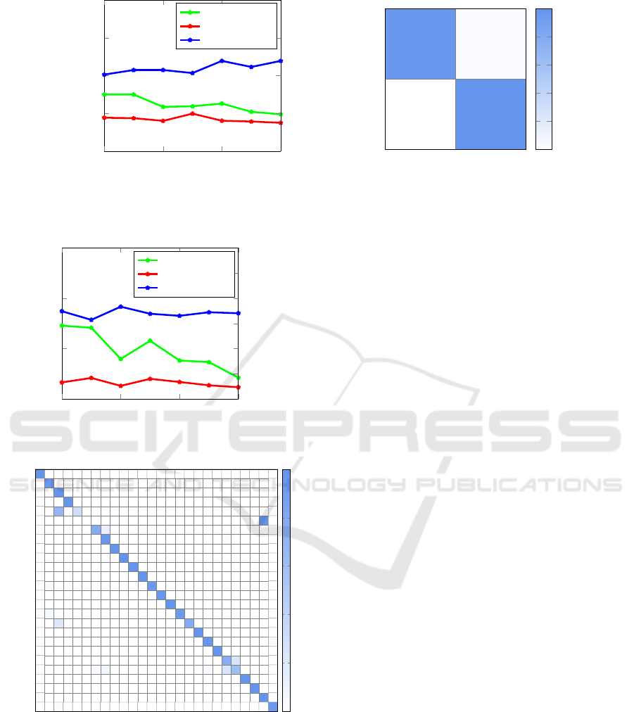
For the binary classification problem in experi-
ment 1, we obtained an accuracy of 98.39%, while the
multiclass problem in experiment 2 yielded an accu-
racy of 94.80%. The results of experiment 1 are sum-
marized in Figure 3, while Figures 4 and 5 give the re-
sults for experiment 2. These experimental results are
comparable to those obtained in (Yajamanam et al.,
2018), and serve to confirm our DL implementation.
We do not have access to the Malimg binary files,
so we are unable to compare the DL results for this
dataset to alternatives that rely on features extracted
directly from executables. Therefore, we next consi-
der the Malicia malware dataset, which will allow us
to compare our image-based DL technique to a sim-
pler k-NN analysis based on non-image features.
For the Malicia dataset, we first generate an image
corresponding to each binary executable sample in the
dataset, as discussed in Section 2.3. Then we per-
form the analogous experiments to 1 and 2, above, but
ForSE 2019 - 3rd International Workshop on FORmal methods for Security Engineering
722

0 2 4
6
0.00
0.05
0.10
0.15
0.20
Epoch
Loss
Training loss
Evaluation loss
0 2 4
6
0.96
0.97
0.98
0.99
1.00
Epoch
Accuracy
Training loss
Evaluation loss
Accuracy
benign
malware
benign
malware
0.960
0.040
0.002
0.998
0.0
0.2
0.4
0.6
0.8
1.0
(a) Training (b) Confusion matrix
Figure 3: Experiment 1 results.
0 2 4
6
0.10
0.20
0.30
0.40
Epoch
Loss
Training loss
Evaluation loss
0 2 4
6
0.90
0.92
0.94
0.96
0.98
1.00
Epoch
Accuracy
Training loss
Evaluation loss
Accuracy
Figure 4: Experiment 2 training.
Adialer.C
Agent.FYI
Allaple.A
Allaple.L
Alueron.gen!J
Autorun.K
C2LOP.P
C2LOP.gen!g
Dialplatform.B
Dontovo.A
Fakerean
Instantaccess
Lolyda.AA1 Lolyda.AA2 Lolyda.AA3
Lolyda.AT
Malex.gen!J
Obfuscator.AD
Rbot!gen
Skintrim.N
Swizzor.gen!E
Swizzor.gen!I
VB.AT
Wintrim.BX
Yuner.A
benign
Adialer.C
Agent.FYI
Allaple.A
Allaple.L
Alueron.gen!J
Autorun.K
C2LOP.P
C2LOP.gen!g
Dialplatform.B
Dontovo.A
Fakerean
Instantaccess
Lolyda.AA1
Lolyda.AA2
Lolyda.AA3
Lolyda.AT
Malex.gen!J
Obfuscator.AD
Rbot!gen
Skintrim.N
Swizzor.gen!E
Swizzor.gen!I
VB.AT
Wintrim.BX
Yuner.A
benign
1.00
0.96
0.04
1.00
1.00
0.67 0.31 0.03
1.00
0.79
0.14 0.03 0.03
0.97
0.03
1.00
1.00
0.99
0.01
1.00
0.05
0.95
0.03
0.97
1.00
0.06
0.94
0.22 0.78
1.00
0.97
0.03
1.00
0.76 0.24
0.04 0.08 0.04 0.23 0.62
1.00
1.00
1.00
0.04
0.95
0.0
0.2
0.4
0.6
0.8
1.0
Figure 5: Experiment 2 confusion matrix.
using the Malicia samples in place of Malimg. Speci-
fically, we perform the following experiments.
Experiment 3. As in experiment 1, we perform bi-
nary classification of malware versus benign, but
in this case, the malware class consists of all
Malicia samples, as images. The benign set con-
sists of the same 3304 Windows samples that were
used in experiment 1.
Experiment 4. For the corresponding multiclass ver-
sion of this problem, we attempt to classify the
Malicia (image) samples into their respective fa-
milies, with the Windows benign set treated as an
additional “family.”
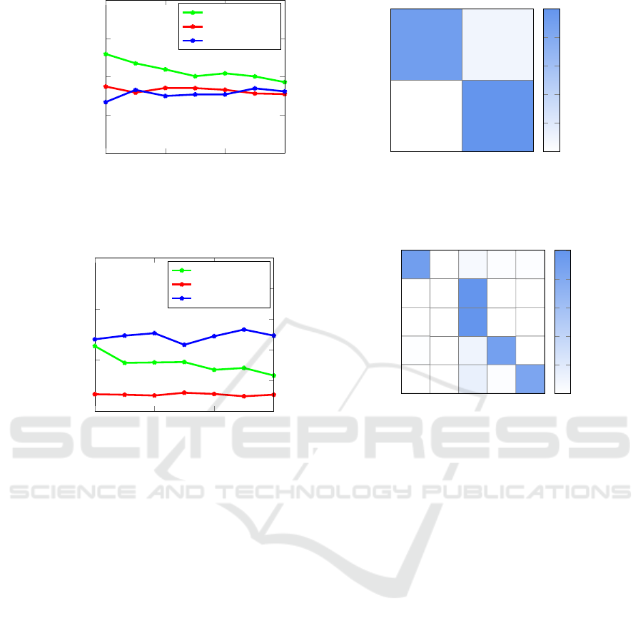
For the binary classification problem in experiment 3,
we obtain an accuracy of 97.61%, while the multi-
class problem in experiment 4 yields a classification
accuracy of 92.93%. The results of experiment 3 are
summarized in Figure 6, while Figure 7 contains the
results of experiment 4. Note that only the four large
Malicia families were used in these experiments, as
the remaining families are severely underrepresented
in the dataset. These results indicate that the multi-
class problem is far more challenging for the Malicia
dataset, as compared to the Malimg dataset. Recall
that there are 26 classes in the Malimg classification
experiment, but only five classes in the corresponding
Malicia experiment, yet we obtain a lower multiclass
accuracy on the Malicia samples.
Next, we compare our DL approach to a simpler
strategy based on k-NN. We extract non-image featu-
res from the Malicia binaries and the benign set, as
discussed in Section 2.4. Then we carry out binary
and multiclass experiments. Specifically, we perform
the following k-NN experiments.
Experiment 5. For this binary classification expe-
riment, we deal with malware and benign sets,
where the malware class consists of Malicia sam-
ples. In this case, non-image features are extrac-
ted directly from the malware binaries. The be-
nign set again consists of the 3304 Windows sam-
ples, and the same non-image features have been
extracted from these samples.
Experiment 6. In the corresponding multiclass ex-
periment, we attempt to categorize the Malicia
Transfer Learning for Image-based Malware Classification
723

0 2 4
6
0.00
0.05
0.10
0.15
0.20
Epoch
Loss
Training loss
Evaluation loss
0 2 4
6
0.96
0.97
0.98
0.99
1.00
Epoch
Accuracy
Training loss
Evaluation loss
Accuracy
benign
malware
benign
malware
0.91 0.09
1.00
0.0
0.2
0.4
0.6
0.8
1.0
(a) Training (b) Confusion matrix
Figure 6: Experiment 3.
0 2 4
6
0.20
0.40
0.60
0.80
Epoch
Loss
Training loss
Evaluation loss
0 2 4
6
0.88
0.90
0.92
0.94
0.96
0.98
Epoch
Accuracy
Training loss
Evaluation loss
Accuracy
benign
securityshield
winwebsec
zbot
zeroaccess
benign
securityshield
winwebsec
zbot
zeroaccess
0.91
0.06 0.02 0.02
1.00
1.00
0.01 0.10
0.89
0.14 0.02 0.84
0.0
0.2
0.4
0.6
0.8
1.0
(a) Training (b) Confusion matrix
Figure 7: Experiment 4.
samples into their respective families, with the
Windows benign set treated as a yet another “fa-
mily.” As above, here we only use the four large
Malicia families which, together with the benign
set, gives us a total of five distinct classes.
As mentioned above, we selected k-NN for these ex-
periments because we want to establish a baseline
by which to compare the performance of our image-
based DL approach. We also want to use non-image
features in this alternative analysis, as this provides
some additional insight into the value of treating mal-
ware samples as images.
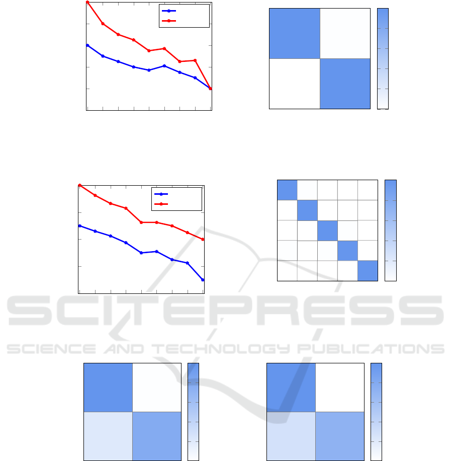
Interestingly, k-NN outperforms DL, achieving an
impressively high accuracy of 99.60% in the binary
classification problem, while a similarly high accu-
racy of 99.43% is attained in the multiclass problem.
Figures 8 and 9, respectively, summarize the results
of experiment 5 and experiment 6. Note that the mul-
ticlass result in experiment 6 is particularly strong, gi-
ven that there are five classes under consideration, in-
cluding a benign set. In contrast, our image-based DL
technique yielded substantially worse results, with an
accuracy of less than 93% on this same dataset.
Next, we attempt to quantify the robustness and
generalizability of our DL (image-based) technique
in comparison to our k-NN (exe-based) classification
strategy. For the DL and k-NN cases, denoted here
as experiments 7 and 8, respectively, we attempt to
classify samples as malware or benign, based on sam-
ples belonging to families that the models have not
been trained to detect. This can be viewed as simula-
ting zero-day malware, that is, malware that was not
available during the training phase. Specifically, we
performed the following zero-day experiments.
Experiment 7. We test our DL approach for the bi-
nary classification of zero-day malware versus be-
nign, where the malware training set consists of
all samples in the four large Malicia families.
The benign training set consists of 3304 Windows
samples. To simulate zero-day malware, the test
set consists of all of the small families in the
Malicia dataset. In addition, to ensure that unfa-
miliar benign binaries did not lead to a high false
positive rate, we used 704 Cygwin binaries as our
benign test set.
ForSE 2019 - 3rd International Workshop on FORmal methods for Security Engineering
724

1 2 3 4
5 6
7 8 9
0.990
0.992
0.994
0.996
0.998
1.000
Number of neighbors (k)
Accuracy
Testing
Training
benign
malware
benign
malware
0.99
0.01
1.00
0.0
0.2
0.4
0.6
0.8
1.0
(a) Determining optimal k (b) Confusion matrix
Figure 8: Experiment 5.
1 2 3 4
5 6
7 8 9
0.984
0.988
0.992
0.996
1.000
Number of neighbors (k)
Accuracy
Testing
Training
benign
securityshield
zeroaccess
zbot
winwebsec
benign
securityshield
zeroaccess
zbot
winwebsec
0.99
0.01
1.00
0.99
0.01
0.01 0.01
0.98
1.00
0.0
0.2
0.4
0.6
0.8
1.0
(a) Determining optimal k (b) Confusion matrix
Figure 9: Experiment 6.
benign
malware
benign
malware
0.99
0.01
0.21
0.79
0.0
0.2
0.4
0.6
0.8
1.0
benign
malware
benign
malware
1.00
0.28 0.72
0.0
0.2
0.4
0.6
0.8
1.0
(a) DL results (b) k-NN results
Figure 10: Zero-day simulations (experiments 7 and 8).
Experiment 8. For our corresponding k-NN experi-
ments, we use the same datasets as in experi-
ment 7. And, as above, to simulate zero-day mal-
ware, the malware test set consists of all of the
small families in the Malicia dataset, and the be-
nign test set consists of the 704 Cygwin samples.
Our image-based DL model performed reasona-
bly well in this zero-day simulation, correctly identi-
fying 79% of the malware samples, with a low false
positive rate of 1%. However, our DL model has a
high false negative rate, as illustrated in Figure 10 (a).
With k-NN, we achieve broadly similar, but somew-
hat worse results, as can be seen from the confusion
matrix in Figure 10. These zero-day experiments indi-
cate that image-based DL models generalize somew-
hat better than a more straightforward k-NN model.
This is a potentially an advantage for image-based DL
Transfer Learning for Image-based Malware Classification
725

models in the malware realm, as detecting zero-day
malware is the holy grail in the AV field. However,
the simplicity and ease of training k-NN models could
be a major advantage in some situations.
5 CONCLUSION
In this paper, we treated malware binaries as images
and classified samples based on pre-trained deep lear-
ning image recognition models. We compared these
image-based deep learning (DL) results to a simpler
k-nearest neighbor (k-NN) approach based on a more
typical set of static features. We carried out a wide
variety of experiments, each representing a different
combination of dataset, classification level, and lear-
ning technique. The multiclass experiments were par-
ticularly impressive, with high accuracy attained over
a large number of malware families.
Our DL method overall delivered results compara-
ble to previous work, yet it was outperformed by the
much simpler k-NN learning technique in some cases.
The image-based DL models did outperform k-NN in
simulated zero-day experiments, which indicates that
this DL implementation better generalizes the training
data, as compared to k-NN. This is a significant point,
since zero-day malware, arguably, represents the ulti-
mate challenge in malware detection.
There are many promising avenues for future
work related to image-based malware analysis. For
example, it seems likely that a major strength of any
image-based strategy is its robustness. Consequently,
additional experiments along these lines would be
helpful to better quantify this effect.
REFERENCES
Austin, T. H., Filiol, E., Josse, S., and Stamp, M. (2013).
Exploring hidden Markov models for virus analysis:
A semantic approach. In 46th Hawaii International
Conference on System Sciences, HICSS 2013, Wai-
lea, HI, USA, January 7-10, 2013, pages 5039–5048.
IEEE Computer Society.
Baysa, D., Low, R. M., and Stamp, M. (2013). Structural
entropy and metamorphic malware. Journal of Com-
puter Virology and Hacking Techniques, 9(4):179–
192.
Damodaran, A., Troia, F. D., Visaggio, C. A., Austin, T. H.,
and Stamp, M. (2017). A comparison of static, dyna-
mic, and hybrid analysis for malware detection. Jour-
nal of Computer Virology and Hacking Techniques,
13(1):1–12.
Fast.ai (2018). Fast.ai lectures. https://course.fast.ai/
lessons/lessons.html.
He, K., Zhang, X., Ren, S., and Sun, J. (2016). Deep re-
sidual learning for image recognition. In 2016 IEEE
Conference on Computer Vision and Pattern Recogni-
tion, CVPR 2016, pages 770–778.
Machine Learning (2018). Machine learning: Github repo-
sitory. https://github.com/tuff96/Malware-detection-
using-Machine-Learning.
Nappa, A., Rafique, M. Z., and Caballero, J. (2015). The
Malicia dataset: Identification and analysis of drive-
by download operations. International Journal of In-
formation Security, 14(1):15–33.
Nataraj, L., Karthikeyan, S., Jacob, G., and Manjunath, B.
(2011). Malware images: Visualization and automatic
classification. In Proceedings of the 8th International
Symposium on Visualization for Cyber Security, Viz-
Sec ’11.
PE File (2018). Pe file: Github repository. https://github.
com/erocarrera/pefile.
Pedregosa, F., Varoquaux, G., Gramfort, A., Michel, V.,
Thirion, B., Grisel, O., Blondel, M., Prettenhofer, P.,
Weiss, R., Dubourg, V., Vanderplas, J., Passos, A.,
Cournapeau, D., Brucher, M., Perrot, M., and Duche-
snay, E. (2011). Scikit-learn: Machine learning in py-
thon. J. Mach. Learn. Res., 12:2825–2830.
Singh, T., Troia, F. D., Visaggio, C. A., Austin, T. H., and
Stamp, M. (2016). Support vector machines and mal-
ware detection. Journal of Computer Virology and
Hacking Techniques, 12(4):203–212.
Smith, L. N. (2015). Cyclical learning rates for training
neural networks. https://arxiv.org/abs/1506.01186.
Stamp, M. (2017). Introduction to Machine Learning with
Applications in Information Security. Chapman and
Hall/CRC, Boca Raton.
Toderici, A. H. and Stamp, M. (2013). Chi-squared distance
and metamorphic virus detection. Journal of Compu-
ter Virology and Hacking Techniques, 9(1):1–14.
Wong, W. and Stamp, M. (2006). Hunting for metamorphic
engines. Journal in Computer Virology, 2(3):211–229.
Yajamanam, S., Selvin, V. R. S., Troia, F. D., and Stamp,
M. (2018). Deep learning versus gist descriptors for
image-based malware classification. In Proceedings
of the 4th International Conference on Information
Systems Security and Privacy, ICISSP 2018, pages
553–561.
ForSE 2019 - 3rd International Workshop on FORmal methods for Security Engineering
726