Smart General Variable Neighborhood Search with Local Search based

on Mathematical Programming for Solving the Unrelated Parallel

Machine Scheduling Problem

Marcelo Ferreira Rego

1,2

and Marcone Jamilson Freitas Souza

Universidade Federal de Ouro Preto (UFOP), Programa de P

os-Graduac¸

ao em Ci

encia da Computac¸

ao,

35.400-000, Ouro Preto, Minas Gerais, Brazil

Universidade Federal dos Vales do Jequitinhonha e Mucuri (UFVJM),

Keywords:

Unrelated Parallel Machine Scheduling, Makespan, VNS, Metaheuristic, Mathematical Programming.

Abstract:

This work addresses the Unrelated Parallel Machine Scheduling Problem in which machine and job sequence-

dependent setup time are considered. The objective is to minimize the makespan. For solving it, a Smart

General Variable Neighborhood Search algorithm is proposed. It explores the solution space through ﬁve

strategies: swap of jobs in the same machine, insertion of job in the same machine, swap of jobs between

machines, insertion of jobs to different machines and an application of a Mixed Integer Linear Programming

formulation to obtain optimum scheduling on each machine. The ﬁrst four strategies are used as shaking mech-

anism, while the last three are applied as local search through the Variable Neighborhood Descent method.

The proposed algorithm was tested in a set of 810 instances available in the literature and compared to three

state-of-the-art algorithms. Although the SGVNS algorithm did not statistically outperform them in these

instances, it was able to outperform them in 79 instances.

1 INTRODUCTION

The Unrelated Parallel Machine Scheduling Problem

with Setup Times (UPMSP-ST) consists of

scheduling a set N of n independent jobs on a

set M of m unrelated parallel machines. Each job

j ∈ N must be processed for exactly one of the

machines, and requires a processing time p

i j

to be

processed in machine i ∈ M. Each machine can

process only one job at a time. In addition, job

execution requires a setup time S

i jk

, which depends

on the machine i and the sequence in which job j and

k will be processed. In this work the objective is to

minimize the makespan.

The study of the UPMSP-ST is relevant due to

its theoretical and practical importance. From a

theoretical point of view, it attracts the interest of

researchers because it is NP-hard. In practical, it

is found in a large number of industries, such as

the textile industry (Lopes and de Carvalho, 2007).

According to (Avalos-Rosales et al., 2013), in a lot

of situations where there are different production

capacities, the setup time of machine depends on

the previous job to be processed (Lee and Pinedo,

1997). This situation is also found in manufacture

of chemical products, where the reactors must be

cleaned between handling of two mixture; however,

the time required for cleaning depends on the jobs that

were previously completed (Tran et al., 2016).

In this work a hybrid algorithm, based on the

General Variable Neighborhood Search – GVNS

(Mladenovi

c et al., 2008) is proposed. It explores the

solution space through ﬁve strategies: swap of jobs

in the same machine, insertion of job in the same

machine, swap of jobs between machines, insertion

of jobs to different machines and an application

of a Mixed Integer Linear Programming (MILP)

formulation to obtain optimum scheduling on each

machine. The ﬁrst four strategies are used as

shaking mechanism, while the last three are applied

as local search through the Variable Neighborhood

Descent. This algorithm was able to outperform three

state-of-art algorithms in 79 among 810 instances

used for testing.

The remainder of this paper is organized as

follows. Section 2 gives a brief review of the

literature. In Section 3 a mathematical programming

formulation for the problem is presented. In Section 4

Rego, M. and Souza, M.

Smart General Variable Neighborhood Search with Local Search based on Mathematical Programming for Solving the Unrelated Parallel Machine Scheduling Problem.

DOI: 10.5220/0007703302870295

In Proceedings of the 21st International Conference on Enterprise Information Systems (ICEIS 2019), pages 287-295

ISBN: 978-989-758-372-8

287

the proposed algorithm is detailed. The results are

presented in Section 5, while in Section 6 the work is

concluded.

2 RELATED WORK

(Arnaout et al., 2014) proposed a two-stage

Ant Colony Optimization algorithm (ACOII) for

minimizing the makespan in the UPMSP-ST. This

algorithm is an enhancement of the ACOI algorithm

that was introduced in (Arnaout et al., 2010). An

extensive set of experiments was performed to verify

the quality of the method. The results proved the

superiority of the ACOII in relation to the other

algorithms with which it was compared.

(Tran et al., 2016) addressed the UPMSP-ST

having as objective the minimization of the makespan.

The authors introduced a new mathematical

formulation, which provides better dual bounds

that are more efﬁcient to ﬁnd the optimum solution.

The computational experiments showed that it is

possible to solve larger instances than it was possible

to solve with other previously existing formulations.

A variant of the Large Neighborhood Search

metaheuristic, using Learning Automata to adapt the

probabilities of using removal and insertion heuristics

and methods, named LA-ALNS, is presented in (Cota

et al., 2017). The algorithm was used to solve

instances of up to 150 jobs and 10 machines. The

LA-ALNS was compared with three other algorithms

and the results show that the developed method

performs best in 88% of the instances. In addition,

statistical tests indicated that LA-ALNS is better than

the other algorithms found in the literature.

The UPMSP-ST was dealt in (Fanjul-Peyro and

Ruiz, 2010), where the objective was to minimize

the makespan. Seven algorithms were proposed: IG,

NSP, VIR, IG+, NSP+, VIR+ and NVST-IG+. The

ﬁrst three are the base algorithms. The following

three are improved versions of these latest algorithms.

Finally, the last algorithm is a combination of the

best ideas from previous algorithms. These methods

are mainly composed of a solution initialization,

a Variable Neighborhood Descent – VND method

(Mladenovi

c et al., 2008) and a solution modiﬁcation

procedure. Tests were performed with 1400 instances

and it was showed that the results were statistically

better than the algorithms previously considered

state-of-the-art, that is, (Mokotoff and Jimeno, 2002)

and (Ghirardi and Potts, 2005).

A Genetic Algorithm was proposed by (Vallada

and Ruiz, 2011) to solve the UPMSP-ST. The

algorithm includes a fast local search and a new

crossover operator. Furthermore, the work also

provides a mixed integer linear programming model

for the problem. After several statistical analyzes, the

authors concluded that their method provides better

results for small instances and, especially, for large

instances, when compared with other methods of the

literature at the time (Kurz and Askin, 2001; Rabadi

et al., 2006).

3 MATHEMATICAL MODEL

This Section provides a Mixed Integer Linear

Programming (MILP) model for the problem from

(Tran et al., 2016). Assume the following parameters:

• p

: processing time of job j on machine i.

• S

i jk

: setup time required for processing job k ∈ N

immediately after job j ∈ N on machine i ∈ M.

• V : a very large real number.

For describing the model, consider the following

decision variables:

i jk







1, if job j immediately precedes job k

on machine i

0, otherwise

= Completion time of job j

= Completion time of machine i.

max

= Maximum completion time

The objective function is given by Equation (1):

min C

max

, (1)

and the constraints are given by Equations (2)-(10):

∑

i∈M

∑

j∈N∪{0},

j6=k

i jk

= 1, ∀k ∈ N, (2)

∑

i∈M

∑

k∈N∪{0},

j6=k

i jk

= 1, ∀ j ∈ N, (3)

∑

k∈N∪{0},

k6= j

i jk

∑

h∈N∪{0},

h6= j

ih j

,∀ j ∈ N, ∀i ∈ M, (4)

> C

+ S

i jk

+ p

−V (1 − x

i jk

∀ j ∈ N ∪ {0},∀k ∈ N, j 6= k,∀i ∈ M, (5)

∑

j∈N

i0 j

6 1, ∀i ∈ M, (6)

= 0 (7)

∑

j∈N∪{0},

j6=k

∑

k∈N

i jk

+ p

i jk

= O

, ∀i ∈ M, (8)

6 C

max

, ∀i ∈ M, (9)

ICEIS 2019 - 21st International Conference on Enterprise Information Systems

288

i jk

∈ {0,1},∀ j ∈ N ∪ {0},∀k ∈ N, j 6= k,∀i ∈ M,

(10)

Equation (1) deﬁnes the objective function of

the problem, which is to minimize the maximum

completion time or makespan. Equations (2) – (10)

deﬁne the constraints of the model. The constraint

set (2) ensures that each job is assigned to exactly

one machine and has exactly one predecessor job.

Constraints (3) deﬁne that every job has exactly one

successor job. Each constraint (4) establishes that if a

job j is scheduled on a machine i, then a predecessor

job h and a successor job k must exist in the same

machine. Constraints (5) ensure a right processing

order. Basically, if a job k is assigned to a machine

i immediately after job j, that is, if X

i jk

= 1, the

completion time C

of this job k) must be greater

than or equal to the completion time C

of job j,

added to setup time between jobs j and k and the

processing time p

of k on machine i. If X

i jk

= 0,

then a sufﬁciently high value V makes this constraint

redundant. With constraint set (6) we deﬁne at most

one job is scheduled as the ﬁrst job on each machine.

Constraints (7) establish that the completion time of

the dummy job is zero. Constraints (8) compute, for

each machine, the time it ﬁnishes processing its last

job. Constraints (9) deﬁne the maximum completion

time.

4 PROPOSED ALGORITHM

4.1 Initial Solution

The initial solution is generated by a constructive

heuristic deﬁned by the Algorithm 1.

Algorithm 1: Initial Solution.

input : M, N

1 foreach k ∈ N do

2 Find the machine i and the position j for the

job k that produces the lowest cost for the

objective function;

3 Insert job k in position j on machine i;

4 end

Algorithm 1 receives the sets M and N of machines

and jobs as parameters, respectively. At each

iteration, a position j on a machine i that provides the

smallest increase in the objective function according

to Eq. (1) is chosen to insert the job k. This process is

repeated for all jobs. The method ends when all jobs

are allocated on some machine.

4.2 Smart GVNS

The proposed algorithm, so-called Smart GVNS, is

based on the General Variable Neighborhood Search

metaheuristic – GVNS (Mladenovi

c et al., 2008).

GVNS explores the solution space of the problem

through systematic neighborhood exchanges and has

the Variable Neighborhood Descent method – VND

(Mladenovi

c and Hansen, 1997) as the local search

method.

In Smart GVNS, the decision for increasing the

perturbation level occurs only after a certain number

of VND applications without improvement in the

quality of the current solution. Smart GVNS was

implemented according to the Algorithm 2:

Algorithm 2: Smart GVNS.

input : stopping criterion, Max, N

1 s

← Initial Solution();

2 ItSameNeigh ← 1;

3 p ← 2;

4 s ← VND(s

,N );

5 while (stopping criterion was not satisﬁed) do

6 s

← Shaking(s, p);

7 s

← VND(s

,N );

8 if ( f (s

) < f (s)) then

9 s ← s

;

10 p ← 2;

11 ItSamePerturb ← 1;

12 end

13 else

14 ItSamePerturb ← ItSamePerturb +1;

15 if (ItSamePerturb > Max) then

16 p ← p + 1;

17 ItSamePerturb ← 1;

18 end

19 end

20 end

21 return s ;

Algorithm 2 receives as input: 1) the stopping

criterion, which in this case was the CPU time t, given

by t = n × 5 seconds, where n is the number of jobs;

2) Max, the maximum number of iterations without

improvement in f (s) with the same perturbation

level; 3) the set N of neighborhoods. In line 1 the

solution s is initialized from the solution obtained

by the procedure deﬁned in Section 4.1. In line 6, a

random neighbor s

is generated from a perturbation

performed according to the procedure deﬁned in

Section 4.2.1. The loop from lines 5-20 is repeated

while the stopping criterion is not satisﬁed. In line 7,

Smart General Variable Neighborhood Search with Local Search based on Mathematical Programming for Solving the Unrelated Parallel

Machine Scheduling Problem

289

Algorithm 3: VND.

input : s, N

1 k ← 1;

2 while (k ≤ 3) do

3 s

← BestNeighbor(s,N

);

4 if ( f (s

) < f (s)) then

5 s ← s

;

6 k ← 1;

7 end

8 else

9 k ← k + 1 ;

10 end

11 end

12 return s ;

a local search on s

using the neighborhood structures

described in Section 4.2.2 is performed. It stops

when it ﬁnds the ﬁrst solution that is better than s

or when the whole neighborhood has been explored.

The solution returned by this local search is attributed

to s

if its value is better than the current solution.

Otherwise, a new neighborhood structure is explored.

4.2.1 Shaking

An important step of a VNS-based algorithm is the

shaking procedure of a solution. This step is applied

so that the algorithm does not get stuck in a same

region of the solution space of the problem and to

explore other regions. For this reason, the algorithm

progressively increases the level of perturbation in a

solution when it is stuck in a local optimum.

In this work, the shaking procedure consists of

applying to the current solution p = 2 moves chosen

among the following: 1) change of execution order of

two jobs of the same machine; 2) change of execution

order of two jobs belonging to different machines; 3)

insertion of a job from a machine into another position

of the same machine and 4) insertion of a job from one

machine into a position of another machine.

It works as follows: p independent moves are

applied consecutively on the current solution s,

generating an intermediate solution s

. This solution

is, then, reﬁned by the VND local search method

(line 7 of the Algorithm 2). The level of perturbation

p increases after a certain number of attempts to

explore the neighborhood without improvement in

the current solution. This limit is controlled by the

variable Max. When p increases, then p random

moves (chosen from those mentioned above) are

applied to the current solution. Whenever there is an

improvement in the current solution, the perturbation

returns to its lowest level, that is, p = 2.

The operation of each type of perturbation is

detailed below:

Swap in the Same Machine: The process of

perturbation by swap of jobs on the same

machine consists in randomly choosing two jobs

and j

that are, respectively, in the positions

x and y of a machine i, and allocate j

in the

position y and j

in the position x of the same

machine i.

Swap between Different Machines: This

perturbation consists in randomly choosing

a job j

that is in the position x in a machine i

and another job j

that is in the position y of

the machine i

. Then, job j

is allocated to

machine i

in position y, and job j

is allocated to

machine i

in position x.

Insertion in the Same Machine: The process of the

insertion in the same machine starts with the

random choice of a job j

that is initially in the

position x of the machine i. Then, a random

choice of another position y of the same machine

is made. Finally, job j

is removed from position

x and inserted into position y of machine i.

Insertion between Different Machines: This

perturbation consists of initially choosing a

random job j

that is in the position x in a

machine i

and a random position y of the

machine i

. After the choice, job j

is removed

from machine i

and inserted into position y of

machine i

4.2.2 Local Search

The exploration of the solution space of the problem

uses three different neighborhood structures: the ﬁrst

one based on job insertion between machines; the

second one in swap of jobs between machines and

the third one in a mathematical heuristic. These

neighborhood structures are described below.

: Insertion Neighborhood Between Machines:

Given a scheduling π = {π

,π

,..., π

} in a

machine i

and a sequencing σ = {σ

,σ

,..., σ

}

in a machine i

, the insertion neighborhood

between machines generates neighboring

solutions as follows. Each job π

is removed from

machine i

and added to machine i

at position y.

The set of insertion moves of every the jobs of a

machine i

in every possible positions of another

machine i

deﬁnes the neighborhood N

(π,σ),

which is composed by |π| × (|σ| + 1) possible

solutions.

Figure 1 illustrates an insertion move of a job π

of a machine i

in the position y of the machine i

ICEIS 2019 - 21st International Conference on Enterprise Information Systems

290

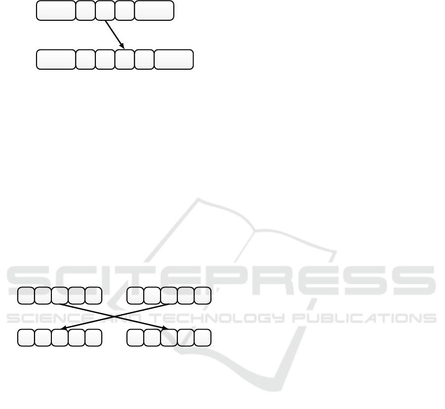
considering a value of x less than y .

x-1

x+1

y-1

y+1

Figure 1: Insertion Move Between Machines i

and i

: Swap Move between Machines: Given a

scheduling π = {π

,π

,..., π

} in a machine

and a scheduling σ = {σ

,σ

,..., σ

} in a

machine i

, the swap move between machines

performed with two jobs π

and σ

moves the

job π

to the position y of the machine i

and the

job σ

to the position x on the machine i

. The

set of swap moves between two machines i

and

deﬁnes the neighborhood N

(π,σ), formed by

|π| ×|σ| solutions.

Figure 2 illustrates the swap between two jobs π

and σ

, which are initially allocated to machines

and i

, respectively. After the swap move, the

job σ

is allocated to machine i

and job π

machine i

x-1

x+1

y-1

y+1

x-1

x+1

y-1

y+1

Figure 2: Swap Move Between Machine i

and i

: Scheduling by Mathematical Programming:

In this local search, the objective is to determine

the best scheduling of the jobs in each machine

by the application of a MILP formulation. This

single machine version that is solved by a MILP

is basically a Traveling Salesman Problem due to

the sequence-dependent setup times.

So, a MILP formulation is solved for the

sequencing problem in each of the machines at

a time. If there is improvement in the current

solution, it returns to the ﬁrst neighborhood (N

If there is no improvement in one machine,

then the model will be applied to the next

machine. If there is no improvement by applying

this formulation to all m machines, then the

exploration is ended to neighborhood N

and also

to the local search. In this case, the local search

returns a local optimum in relation to all three

neighborhoods N

, N

and N

The mathematical formulation given by

Equations (11)–(16) was applied to the jobs

⊆ N of each machine i. The decision variables

are:



1, if job k is processed directly after job j

0, otherwise

max

= Maximum completion time on machine i

min C

max

, (11)

∑

j∈N

∪{0},

j6=k

= 1, ∀k ∈ N

, (12)

∑

k∈N

∪{0},

j6=k

= 1, ∀ j ∈ N

, (13)

∑

j∈N

∪{0}

j6=k

∑

k∈N

i jk

+ p

= C

max

, (14)

∈ {0,1}, (15)

∑

j∈δ

∑

k /∈δ

≥ 1 ∀δ ⊂ N

,δ 6=

0 (16)

Equation (11) deﬁnes the objective function,

which is to minimize the completion time of the

machine i.

Equations (12)–(16) deﬁne the constraints for the

sub-model. Constraints (12) ensure that every

job k has exactly one predecessor job, and the

predecessor job of the ﬁrst job is the dummy

job 0. Constraints (3) ensure that each job k

has a successor job, and the successor of the

last job is the dummy job 0. Constraints (14)

compute the completion time on the machine i.

Constraints (15) deﬁne the domain of the decision

variables. Constraints (16) ensure that there is no

sub-sequencing, therefore, any subset of jobs δ

contained in N

must have at least one link with

another subset complementary to δ. This strategy

is similar to the subtour elimination constraints

for the traveling salesman problem, proposed by

(Bigras et al., 2008).

The mathematical model has a constraint for

each subset of jobs. Thus, in cases where the

scheduling problem has many subsets of jobs, the

model will present a high computational cost. For

this reason, the set of constraints (16) was initially

disregarded from the model. However, the relaxed

model can produce an invalid solution, that is, a

solution containing one or more cyclic sequences.

If this happens, a new set of constraints for each

Smart General Variable Neighborhood Search with Local Search based on Mathematical Programming for Solving the Unrelated Parallel

Machine Scheduling Problem

291

cyclic sequencing is added to the mathematical

model to be solved again. In this new set of

constraints (16), the set δ is formed by the group

of jobs belonging to the cyclic sequencing. This

process is repeated until a valid solution is found.

For illustrating this situation, consider the matrix

below that represents the values of the decision

variables for a problem of a machine with 5 jobs.

Table 1: Example of an invalid solution.

Y 0 1 2 3 4 5

0 0 0 0 0 0 1

1 0 0 1 0 0 0

2 0 1 0 0 0 0

3 1 0 0 0 0 0

4 0 0 0 1 0 0

5 0 0 0 0 1 0

Consider that if Y

= 1 then job j immediately

precedes job k, and that the ﬁrst job of the

sequence is preceded by the dummy job 0. Then

we have the following sequencing: δ

= {5,4,3}

and δ

= {1,2}. In this example, δ

is a cyclic

sequencing. This solution is invalid since there

should be a single sequencing and not two as

can be observed. It is possible to observe that

represents a cyclic sequencing, since job 1

precedes job 2 and this, in turn, precedes job 1.

Thus, a new constraint must be added for any

solution that presents a cyclic sequencing, since

this situation does not meet the Equation (16).

4.3 Parameter Tunning

The implementation of the Smart GVNS algorithm

requires the calibration of two parameters: Max,

which is deﬁned in Algorithm 2, and the time t as

stopping criterion. The maximum execution time

t of the algorithm for each instance was calculated

according to Equation (17):

t = F ×n (17)

where n is the number of jobs of the instance.

In order for tunning the values of these

parameters, the Irace package (L

opez-Ib

nez

et al., 2016) was used. Irace is an algorithm

implemented in R that implements an iterative

procedure having as main objective to ﬁnd the

most appropriate conﬁgurations for an optimization

algorithm, considering a set of instances of the

problem.

We tested the following values for these

parameters: Max ∈ {4, 5, 6, 7, 8, 9, 10} and

F ∈ {4, 5, 6, 7, 8}. The best conﬁguration returned

by Irace was Max = 9 and F = 7. However, as will be

shown later, only the Max parameter was used, since

the criterion of stopping by processing time was ﬁxed

for a more just comparison with other algorithms of

the literature.

5 RESULTS

The Smart GVNS algorithm was coded in C++

language and the tests were performed on a

microcomputer with the following conﬁgurations:

Intel (R) Core (TM) i7 processor with clock frequency

2.4 GHz, 8 GB of RAM and with a 64-bit

Ubuntu operating system installed. The mathematical

heuristic, used as local search, was implemented

using the Gurobi API (Gurobi Optimization, 2018)

for the C++ language.

The proposed algorithm was tested in three sets of

instances available in (Rabadi et al., 2006): Balanced,

Process Domain and Setup Domain. Each set is

formed by 18 groups of instances, and each group

contains 15 instances. In the ﬁrst set, the processing

time and the setup time are balanced. In the second,

the processing time is dominant in relation to the

setup time and in the third, the setup time is dominant

in relation to the processing time.

Tables 2, 3 and 4 present the results of

the proposed Smart GVNS algorithm (denoted by

SGVNS, for simplicity) in these three set of instances.

These tables compare the results of SGVNS with

those of ACOII reported in (Arnaout et al., 2014)

and AIRP and LA-ALNS reported in (Cota et al.,

2017), considering the value of the Relative Percent

Deviation (RPD), which is given by:

RPD

alg

− f

× 100 (18)

where f

alg

is the value of the objective function for

the algorithm alg in relation to the instance l, while

represents the best value for the objective function

obtained in the l-th instance by the ACOI algorithm

as reported in (Arnaout et al., 2014).

As stopping criterion of the Smart GVNS

algorithm and for a fair comparison, the average

execution time of ACOII in (Arnaout et al., 2014) was

used. Their time was divided by 2.37 because our

computer is approximately 2.37 times faster than the

computer used in (Arnaout et al., 2014) according to

(PassMark, 2018). (Cota et al., 2017) also used the

same stopping criterion to present the results of AIRP

and LA-ALNS algorithms.

ICEIS 2019 - 21st International Conference on Enterprise Information Systems

292

In these tables, the ﬁrst and second columns

represent the number of machines and jobs,

respectively. In the subsequent columns is the average

RPD for the ACOI, ACO-II, AIRP, LA-ALNS and

SGVNS algorithms, respectively. The average RPD

presented considers a group of 15 instances.

Table 2: Average RPD in Balanced instances.

m n ACOII AIRP LA-ALNS SGVNS

80 -0.349 0.440 0.191 -0.103

100 -0.306 0.560 0.123 -0.057

120 -0.420 0.440 0.015 -0.181

80 0.747 0.840 0.243 1.287

100 0.739 0.910 0.171 1.395

120 0.428 0.810 0.183 1.137

80 1.682 0.910 0.296 1.855

100 1.481 1.120 0.206 2.146

120 1.028 1.130 0.262 2.309

80 0.012 0.595

100 0.000 0.474

120 0.020 1.002

80 1.739 1.060 0.462 2.790

100 2.854 1.280 0.371 3.073

120 2.270 1.390 0.287 3.282

80 0.017 1.665

100 -0.028 1.335

120 0.036 1.372

Table 3: Average RPD in the Process Domain instances.

m n ACOII AIRP LA-ALNS SGVNS

80 -0,224 0,250 0,119 -0,114

100 0,773 0,370 0,082 -0,076

120 0,619 0,340 0,062 -0,111

80 0,499 0,490 0,160 0,782

100 0,469 0,550 0,106 0,658

120 0,388 0,340 0,129 0,484

80 0,508 0,440 0,364 1,071

100 1,223 0,840 0,185 1,499

120 0,759 0,510 0,160 0,876

80 -0,018 0,333

100 -0,006 0,172

120 0,010 0,238

80 0,894 0,420 0,261 1,900

100 1,849 0,840 0,248 1,910

120 1,487 0,530 0,157 1,460

80 0,026 1,021

100 0,020 0,686

120 -0,004 0,385

According to Tables 2, 3 and 4, the LA-ALNS

algorithm was superior in 27 groups of instances,

while the ACOII algorithm was superior in 21 groups

of instances and the Smart GVNS algorithm was

superior in 5 groups of instances. Considering

the presented results, it is possible to afﬁrm that

the LA-ALNS algorithm obtained the best average

results, even though it was not applied to all the

instances made available in (Rabadi et al., 2006).

Table 4: Average RPD in the Setup Domain instances.

m n ACOII AIRP LA-ALNS SGVNS

80 -0,163 0,220 0,120 -0,102

100 0,597 0,340 0,070 -0,091

120 0,588 0,320 0,067 -0,076

80 0,639 0,440 0,118 0,788

100 0,452 0,580 0,135 0,643

120 0,351 0,490 0,072 0,542

80 0,786 0,590 0,346 1,131

100 1,273 0,820 0,175 1,870

120 0,576 0,510 0,173 1,094

80 -0,025 -0,053

100 -0,006 0,164

120 0,000 0,325

80 0,953 0,650 0,209 2,003

100 1,759 0,790 0,212 1,969

120 1,204 0,580 0,167 1,510

80 0,000 1,285

100 0,012 1,055

120 -0,014 0,906

The proposed algorithm presented a value for

RPD less than 0 in instances with two machines.

If we consider instances with 4 machines, the RPD

was always less than 2, while for instances with up

to 8 machines, the RPD was always less than 3.

For the other instances, the RPD was always less

than 4. These results indicate that the proposed

method obtained a better performance in instances

with fewer machines, in which the solution space

is smaller. In other cases, the method has lower

performance, given the high computational cost of the

mathematical heuristic, which is used as one of the

local search operators.

A hypothesis test was performed to verify if

the differences between the results presented by the

algorithms are statistically signiﬁcant. Therefore, the

following hypothesis test was used:

(

: µ

= µ

: ∃i, j | µ

6= µ

in which µ

, µ

and µ

are the average RPDs for

ACOII, LA-ALNS and Smart GVNS, respectively.

As it was not possible to establish that the samples

do not originate from a population with a normal

distribution, it was decided to use the Kruskal-Wallis

test. It is a nonparametric test used to compare three

or more populations. It tests the null hypothesis that

all populations have the same distribution functions

versus the alternative hypothesis that at least two of

the populations have different distribution functions.

The paired Kruskal-Wallis test for the samples of

the average results of the ICOII, LA-ALNS and Smart

GVNS algorithms returned p-value = 9.866e-05.

Considering that this p-value is much lower than

Smart General Variable Neighborhood Search with Local Search based on Mathematical Programming for Solving the Unrelated Parallel

Machine Scheduling Problem

293

0.05, then the null hypothesis of equality between the

means is rejected and it is concluded that there is

evidence that at least two populations have different

distribution functions.

In order to identify which samples have RPDs

with statistically signiﬁcant differences, the Nemenyi

test (Nemenyi, 1963) was adopted. Table 5 shows the

results with pairwise comparisons. It is a post-hoc

test, that is, a multiple comparison test that is applied

after a test with three or more factors.

Table 5: Results of the Nemenyi test.

ACOII LA-ALNS

LA-ALNS 0.242 –

SGVNS 0.012 9.8e-05

According to Table 5 there is statistically

signiﬁcant difference between our algorithm and

the ACOII and LA-ALNS algorithms. Although

the LA-ALNS algorithm outperformed the ACOII

algorithm in all sets of instances in which they were

compared, except in sets with two machines, there

was no statistical evidence of its superiority.

6 CONCLUSIONS

This work addressed the Unrelated Parallel Machine

Scheduling Problem in which machine and job

sequence-dependent setup time are considered. The

objective is to minimize the makespan.

In order to solve it, a GVNS-based algorithm,

named SGVNS, is proposed. It explores the solution

space of the problem by means of insertion and

exchange moves of jobs in the same machine and in

different machines, as well as by the application of

a mathematical programming formulation to obtain

optimum scheduling on each machine.

The proposed algorithm was tested in 810

instances of the literature and compared to three other

literature methods (ACOII, AIRP and LA-ALNS).

SGVNS behaved better in instances with a small

number of machines, even though the number of jobs

was high.

From a hypothesis test it was possible to obtain

statistical evidence that the result presented by

LA-ALNS and ACOII are signiﬁcantly better than the

Smart GVNS algorithm. Despite this, SGVNS was

superior in 5 groups of instances and able to ﬁnd best

results in 79 of the 810 instances.

In the future we intend to increase the efﬁciency

of our algorithm to make it more competitive. An

alternative is to test other mathematical programming

formulations to perform the local search. Another

alternative is to apply the local search based on

mathematical programming only periodically, since it

consumes a high computational time.

ACKNOWLEDGEMENTS

The authors thank Coordenac¸

ao de Aperfeic¸oamento

de Pessoal de N

ıvel Superior (CAPES) - Finance

Code 001, Fundac¸

ao de Amparo

a Pesquisa

do Estado de Minas Gerais (FAPEMIG, grant

PPM/CEX/FAPEMIG/676-17), Conselho Nacional

de Desenvolvimento Cient

ıﬁco e Tecnol

ogico (CNPq,

grant 307915/2016-6), Universidade Federal de Ouro

Preto (UFOP) and Universidade Federal dos Vales

do Jequitinhonha e Mucuri (UFVJM) for supporting

this research. The authors also thank the anonymous

reviewers for their valuable comments.

REFERENCES

Arnaout, J.-P., Musa, R., and Rabadi, G. (2014). A two-

stage ant colony optimization algorithm to minimize

the makespan on unrelated parallel machines – part

ii: enhancements and experimentations. Journal of

Intelligent Manufacturing, 25(1):43–53.

Arnaout, J.-P., Rabadi, G., and Musa, R. (2010). A two-

stage ant colony optimization algorithm to minimize

the makespan on unrelated parallel machines with

sequence-dependent setup times. Journal of Intelli-

gent Manufacturing, 21(6):693–701.

Avalos-Rosales, O., Alvarez, A. M., and Angel-Bello, F.

(2013). A reformulation for the problem of scheduling

unrelated parallel machines with sequence and ma-

chine dependent setup times. In Proc. of the 23th In-

ternational Conference on Automated Planning and

Scheduling – ICAPS, pages 278–283, Rome, Italy.

Bigras, L.-P., Gamache, M., and Savard, G. (2008). The

time-dependent traveling salesman problem and sin-

gle machine scheduling problems with sequence de-

pendent setup times. Discrete Optimization, 5(4):685–

699.

Cota, L. P., Guimar

aes, F. G., de Oliveira, F. B., and Souza,

M. J. F. (2017). An adaptive large neighborhood

search with learning automata for the unrelated par-

allel machine scheduling problem. In Evolutionary

Computation (CEC), 2017 IEEE Congress on, pages

185–192. IEEE.

Fanjul-Peyro, L. and Ruiz, R. (2010). Iterated greedy

local search methods for unrelated parallel machine

scheduling. European Journal of Operational Re-

search, 207(1):55–69.

Ghirardi, M. and Potts, C. N. (2005). Makespan minimiza-

tion for scheduling unrelated parallel machines: A re-

covering beam search approach. European Journal of

Operational Research, 165(2):457–467.

ICEIS 2019 - 21st International Conference on Enterprise Information Systems

294

Gurobi Optimization, L. (2018). Gurobi optimizer refer-

ence manual. Available at http://www.gurobi.com.

Kurz, M. and Askin, R. (2001). Heuristic scheduling

of parallel machines with sequence-dependent set-up

times. International Journal of Production Research,

39(16):3747–3769.

Lee, Y. H. and Pinedo, M. (1997). Scheduling jobs

on parallel machines with sequence-dependent setup

times. European Journal of Operational Research,

100(3):464–474.

Lopes, M. J. P. and de Carvalho, J. V. (2007). A branch-and-

price algorithm for scheduling parallel machines with

sequence dependent setup times. European journal of

operational research, 176(3):1508–1527.

opez-Ib

nez, M., Dubois-Lacoste, J., P

erez C

aceres, L.,

utzle, T., and Birattari, M. (2016). The irace pack-

age: Iterated racing for automatic algorithm conﬁgu-

ration. Operations Research Perspectives, 3:43–58.

Mladenovi

c, N., Dra

c, M., Kova

cevic-Vuj

c, V., and

Cangalovi

c, M. (2008). General variable neighbor-

hood search for the continuous optimization. Euro-

pean Journal of Operational Research, 191(3):753–

770.

Mladenovi

c, N. and Hansen, P. (1997). Variable neigh-

borhood search. Computers & Operations Research,

24(11):1097–1100.

Mokotoff, E. and Jimeno, J. (2002). Heuristics based on

partial enumeration for the unrelated parallel proces-

sor scheduling problem. Annals of Operations Re-

search, 117(1):133–150.

Nemenyi, P. (1963). Distribution-free Mul-

tiple Comparisons. Available at

https://books.google.com.br/books?id=nhDMtgAACAAJ.

PassMark (2018). Cpu benchmarks. Available at

https://www.cpubenchmark.net/. Acessed on Febru-

ary 12, 2018.

Rabadi, G., Moraga, R. J., and Al-Salem, A. (2006). Heuris-

tics for the unrelated parallel machine scheduling

problem with setup times. Journal of Intelligent Man-

ufacturing, 17(1):85–97.

Tran, T. T., Araujo, A., and Beck, J. C. (2016). Decom-

position methods for the parallel machine scheduling

problem with setups. INFORMS Journal on Comput-

ing, 28(1):83–95.

Vallada, E. and Ruiz, R. (2011). A genetic algorithm for the

unrelated parallel machine scheduling problem with

sequence dependent setup times. European Journal of

Operational Research, 211(3):612–622.

Smart General Variable Neighborhood Search with Local Search based on Mathematical Programming for Solving the Unrelated Parallel

Machine Scheduling Problem

295