Predicting Fault Proneness of Programs with CNN

Kazuhiko Ogawa and Takako Nakatani

The Open University of Japan, 2-11, Wakaba, Mihama-ku, 261-8586, Chiba, Japan

Keywords:

Deep Learning, Convolutional Neural Network, Program Quality, Fault Prone.

Abstract:

There has been a lot of research aimed at improving the quality of software systems. Conventional methods do

have the ability to evaluate the quality of software systems with regard to software metrics. (i.e. complexity,

usability, modiﬁability, etc.) In this paper, we apply one of the deep learning techniques, CNN (Convolutional

Neural Network), in order to infer the fault proneness of a program. The CNN approach consists of three

steps: training, veriﬁcation of the learning quality, and application. In the ﬁrst step, in order to make training

data, we transformed 27 program source codes into 1490 images with colored elements, so that the features of

the images remain. In the second step, we set the goal of the accuracy of machine learning and trained with the

training data. In the third step, we forced the trained system to infer the fault proneness of 692 images, which

were transformed through 5 programs. This paper presents the effectiveness of our approach for improving

the quality of software systems.

1 INTRODUCTION

Software systems have become deeply involved in

our lives as social systems. As a result, systems are

required to satisfy and excel better usability for di-

versiﬁed end users, safety, and security for our so-

cial life. Furthermore, architectural design for quick

and ﬂexible updating has become a common require-

ment. Flexible updating and/or responding means that

the development period becomes shortened. Business

owners also require that the developments be cost-

effective. It is mandatory for developers to improve

the productivity and efﬁciency of their developments,

along with the quality of their products with regard to

the tradeoff between the increasing requirements and

the cost-effectiveness in time for delivery.

Researchers and developers developed various

technologies to cope with human errors in analy-

sis, design, and implementation. Finding and ﬁx-

ing these errors in the early stage of development

is one of the important goals. In order to reduce

the complexity of a given software, various system

construction methodologies are also proposed. The

most famous and inﬂuential one is the object-oriented

software construction methodology (Mayer, 2000).

Multi-agent systems also contribute to the ease of

large scale software construction (Shehory and Sturm,

2016). Kambayashi and Takimoto (Kambayashi and

Takimoto, 2005) demonstrated that multiple agents

have introduced modularity, reconﬁgurability and ex-

tensibility to control systems, and simpliﬁed the de-

velopment of such software systems. Even though the

ongoing proposal of new methodologies are effective,

the essential part of reliable software construction is

in ﬁnding defects within the software. After all, soft-

ware construction is reliant on human ability.

Practically, we know that we cannot ﬁx all errors

and defects through testing, and furthermore, some

unknown defects sometimes cause fatal faults. We ap-

ply a CNN (Convolutional Neural Network) model to

improve the quality of software. We call this system

as a CNN based bug inference system (the CNN-BI

system for short).

The purpose of this paper is to present the ef-

fectiveness of the CNN approach to predict the fault

proneness of programs. CNN is one of the mecha-

nisms of deep learning, has been successful in the

ﬁeld of image recognition, or inference as based on

images. We expect the CNN-BI system to extract fea-

tures of fault proneness of programs throughout the

training, as the features of fault proneness of a pro-

gram must be presented in the images. Furthermore,

we expect the following effectiveness of the CNN ap-

proach.

• The source codes that cause fault must have pecu-

liar features.

The CNN approach may be able to ﬁnd the fea-

tures in the colored program images rather than in

Ogawa, K. and Nakatani, T.

Predicting Fault Proneness of Programs with CNN.

DOI: 10.5220/0007704303210328

In Proceedings of the 11th International Conference on Agents and Artiﬁcial Intelligence (ICAART 2019), pages 321-328

ISBN: 978-989-758-350-6

321

monochrome images.

• If the CNN model can infer the fault proneness of

a program, we will be able to review and ﬁx the

program faults regardless of its completion.

Thus, we utilize source code images to train a CNN

model in order to infer the fault proneness of pro-

grams.

The research questions of this paper are as fol-

lows:

• RQ1: Can a CNN extract features of fault prone-

ness from images of programs?

• RQ2: If the CNN cannot infer fault proneness,

what kinds of defects are missing?

• RQ3: Is the accuracy of the inference acceptable?

How can accuracy be improved?

In order to get the answers to these research questions,

we need to categorize elements of program source

codes and transform programs into images that the

CNN-BI system reads, which was carried out as fol-

lows. We transformed program source codes into im-

ages with colored elements to train the CNN-BI sys-

tem. Since we did not have an acceptable number

of training data sets, transfer learning (Weiss et al.,

2016) was applied. Before the evaluation of the CNN,

we train the CNN with images of fault prone and cor-

rect programs. Supervised learning was selected as

the CNN’s learning style, since the goal of inference

was to conclude whether the program is fault prone

or not. After the training, the CNN-BI system was

evaluated as to whether the system could predict fault

proneness of a program.

The remainder of this article is structured as fol-

lows. Section 2 presents related work. Section 3 de-

scribes a case study. In Section 4, we discuss the ﬁnd-

ings and their implications. Section 5 concludes.

2 RELATED WORK

There are a lot of methods that improve the quality of

software. Techniques utilizing statistical methods are

popularly applied, since the statistical approach can

visualize the quality of software. If qualitative infor-

mation can be presented quantitatively, we can com-

pare the qualitative characteristics of programs with

the quantitative data. We will be able to observe and

control the quality of software quantitatively to im-

prove the quality of software.

Cyclomatic complexity was introduced by Mc-

Cabe in 1976 (McCabe, 1976). There is a strong

correlation coefﬁcient between the cyclomatic num-

ber and the number of defects. Therefore, when a

program is measured with a big cyclomatic number,

it implies that the program is more complex than pro-

grams with smaller cyclomatic numbers. The quan-

titatively presented “relatively complex” programs

need to be carefully reviewed. After a decade, mul-

tiple paradigms began to be applied. For object-

oriented software, Chidamber and Kemerer intro-

duced metrics to measure complexity based on cou-

pling and cohesion, readability, understandability,

modiﬁability, etc. (Chidamber and Kemerer, 1994).

Their set of metrics is known as CK metrics. Zimmer-

mann also introduced a defect prediction model (Zim-

mermann et al., 2007). These methods are based on a

quantitative approach to evaluate the quality of soft-

ware systems.

The quantitative approach needs evaluation crite-

ria. Lorenz and Kidd presented empirical data for typ-

ical metrics as criteria of the quality of object-oriented

programs (Lorenz and Kidd, 1994). Their intention

was that if the measurement of a program is not within

the “normal” range, the program must be reviewed.

This means that the metrics do not ﬁnd defects or er-

rors of programs. Furthermore, even though testing

is effective in improving the quality of programs, it

cannot discover all errors. One of the difﬁcult points

of improving the quality of programs is that all of the

defects do not occur in the complex program. We em-

ployed another approach to decide which part to re-

view intensively. The CNN approach may be able to

ﬁnd defects that occur not only by the complexity of

the program, but also by the structural feature of the

program.

After the google cat (Le et al., 2012), research

and application examples of deep learning have in-

creased. There are studies that have applied deep

learning to software quality evaluation. For example,

Morisaki applied deep learning to evaluate the read-

ability of software in order to control the quality of

software (Morisaki, 2018). Kondo et al. utilized deep

learning to cope with the delay of feedback from static

code analysis (Kondo et al., 2018). Yang et al. (Yang

et al., 2015) also applied deep learning to observe

software changes and proposed W-CNN rather than

CNN. We evaluate the CNN-BI system whether it can

predict fault proneness of programs.

3 CASE STUDY

In order to evaluate an inference of fault proneness

of programs with deep learning, we analyzed the ef-

fectiveness of the inference qualitatively and quantita-

tively. In this section, we look at a case in which CNN

has been applied in order to infer the fault proneness

HAMT 2019 - Special Session on Human-centric Applications of Multi-agent Technologies

322

of programs. For training the CNN-BI system, we

utilized TensorFlow and KERAS that are provided by

Google with Python on Windows 10 Home. The de-

velopment system conﬁguration was Core i7 - 6700 K

for CPU, 8 GB for MainMemory, and Geforce 980 Ti

for GPU.

3.1 Overview

The case shown in this paper is a project with ﬁfteen

developers, who worked for a period of one year. The

number of programs developed was 575. They used

VisualBasic2008.

The images of programs were created by the fol-

lowing steps.

1. We collected source codes as training data.

We randomly selected 27 programs from 575 pro-

grams.

2. Each element in the statements was color coded

based on the following categories;

• instruction: blue

• reserved word: orange

• comment: green

• module name: bold face, green

• global variable name: bold face, blue

• local variable name: black

• control name: pink

• user deﬁned function name, subroutine name:

bold face, red

• user deﬁned type name: purple

• string: brown

3. We divided each module program into subpro-

grams with approximately thirty lines of code.

“One function must be developed within thirty

lines of code” is one of the coding conventions

in the project.

4. The image of each subprogram was created in B5

size horizontals.

We got 1490 images as training data. In other

words, each image represents a program frag-

ment. The fault proneness would be trained and

inferred for each image.

5. The training data for supervised learning was cat-

egorized into two groups; “with fault” and “with-

out fault,” and were labeled “BUG” or “OK” re-

spectively.

6. We trained the CNN-BI system with the training

data.

We used VGG 16 (VGG ILSVRC 16 layers)

which is a learned model of ImageNet as the

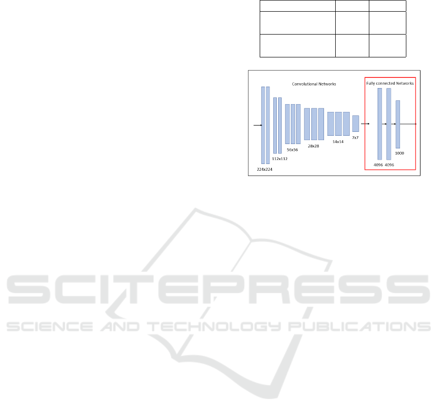
Table 1: The amount of training data and veriﬁcation data.

Data Category Label #cases

Training data OK 945

BUG 545

Veriﬁcation data OK 213

BUG 109

Figure 1: VGG 16 model diagram.

learning model of the CNN-BI system. The

VGG16 has 16 layers in total, including 13 con-

volution layers, and 3 full connected layers. The

VGG16 has learned about object recognition of

1000 categories.

Figure 1 shows the structure of the VGG16. The

convolution layers was reused as the learned mod-

els of the CNN-BI system. We trained the full

connected layers with the training data in order

to infer the fault proneness of program fragments,

then classiﬁed them into two categories based on

the presence or absence of defects, and output the

inference results.

Figure 2 shows the model of the all full connected

layers that we trained. Such a learning method

is called transfer learning. Transfer leaning helps

us apply the trained model from a certain area to

another area in which we have a limited amount

of data. Hence, we utilized transfer learning and

evaluate the quality of source codes with the lim-

ited amount of training data.

7. Similarly, we derived 322 images as veriﬁcation

data.

Here, the veriﬁcation data was utilized to verify

the adequacy of the learning.

8. We veriﬁed the CNN-BI system with the veriﬁca-

tion data.

Underﬁtting and overﬁtting were categorized as

inadequate learning.

The amount of training and veriﬁcation data is shown

in Table 1.

Predicting Fault Proneness of Programs with CNN

323

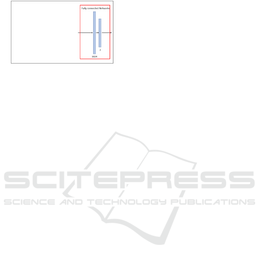
Figure 2: Modiﬁed model of the full connected layers.

3.2 Results of Training and Veriﬁcation

We set the objective of the machine learning with the

goal of achieving 85% of the accuracy. We weighted

the training data (Japkowicz, 2000) so that the num-

ber of cases belonging to the two categories would be

balanced. The training process with the learning data

is shown in Figure 3.

The x axis and y axis of the ﬁgure shown on the

left hand side represent the number of epochs, and the

number of losses respectively. Similarly, the y axis

of the ﬁgure shown on the right hand side represents

the accuracy of the learning. Here, one “epoch” is

one full training cycle of learning. Thus, x axis rep-

resents the number of training cycles. For example,

100 epochs mean that the machine learning cycle has

iterated 100 times.

In the ﬁgures, the blue lines represent the loss and

accuracy for training. On the other hand, red lines

represent the loss and accuracy for validation. We

have done 100 epochs of training. As shown in the

Figure 3a, the loss drops to the right. Figure 3b rep-

resents the accuracy, and rises to the right. Because

the lower loss and higher accuracy represents a bet-

ter CNN model, the training was done successfully

without overﬁtting nor underﬁtting. After the train-

ing, the loss and accuracy rates reached to 19.04%

and 82.97% respectively.

The ﬁrst goal of the accuracy of our training was

85% or greater. However, our achieved accuracy rate

was 82.97%, which was lower than our targeted accu-

racy, but we do retrain the ability to train CNN with-

out overﬁtting or underﬁtting. Hence, we decided to

apply the trained CNN to infer the fault prone pro-

gram fragments.

3.3 Results of Inference

Thus, we applied the trained CNN-BI system to infer

the fault proneness of program fragments. Constraints

of the inference were as follows.

1. Source codes that were used to train the CNN-BI

system should not be applied for the inference.

2. Source codes that we utilized for the inference

should be programs that had not yet been cor-

rected or modiﬁed to resolve the faults.

3. The number of “OK” and “BUG” images should

not deviate considerably from the percentage of

training data. This constraint was intended to

make the inference result be comparable and ver-

iﬁable with the training data.

The inference was carried out for 692 images.

Then, we were able to get a judgement for each im-

age. Figure 4 shows an example of the results of an

inference. In Figure 4, the name of a jpeg ﬁle is shown

at the top of the ﬁgure. The following image is the

thumbnail of the inferred image. The inferred result

is shown under the image. Since the training had been

done with two labels: “OK” and “BUG”, the label

whose possibility is larger than that of the other la-

bel is shown as the inferred result. In this example,

“Result: OK” represents that this program was not in-

ferred as a fault prone program. On the other hand, if

the result is shown as “Result: BUG”, the image was

inferred as a fault prone program. The bottom line of

the ﬁgure represents the probability of BUG and that

of OK. The results of the example are as follows, the

probability of BUG was approximately 0.41, and that

of OK was approximately 0.59.

As we mentioned above, the inference data were

program fragments before ﬁxing any defects. In or-

der to discuss the precision and recall to evaluate the

results of the inferences, we investigated the modiﬁ-

cation history of the programs. If a program was not

modiﬁed, the label of all of the images of the program

must be “OK.” Contrarily, if the program had been

modiﬁed at least once, the labels of the images cor-

responded to the modiﬁed fragments of the program,

and so, were “BUG”, however, the labels of other im-

ages were “OK.” If an inferred label was matched to

the actual label, the result of the inference was cor-

rect.

Each program is plotted in Figure 5 with the num-

ber of images on the x axis and the number of defects

on the y axis. As the number of images represents the

size of a program, the inclination of the line that con-

nects each plot from the origin represents the quality

of the program. For example, if the slope is large, the

quality of the program is low. There are two layered

data in the ﬁgure. We categorized programs into three

layers. Programs categorized in layer 1 were more

fault prone than programs in layer 2.

In order to evaluate the inferred results, we exam-

ined precision and recall with the actual label of each

program fragment. The inferred results are plotted in

HAMT 2019 - Special Session on Human-centric Applications of Multi-agent Technologies

324

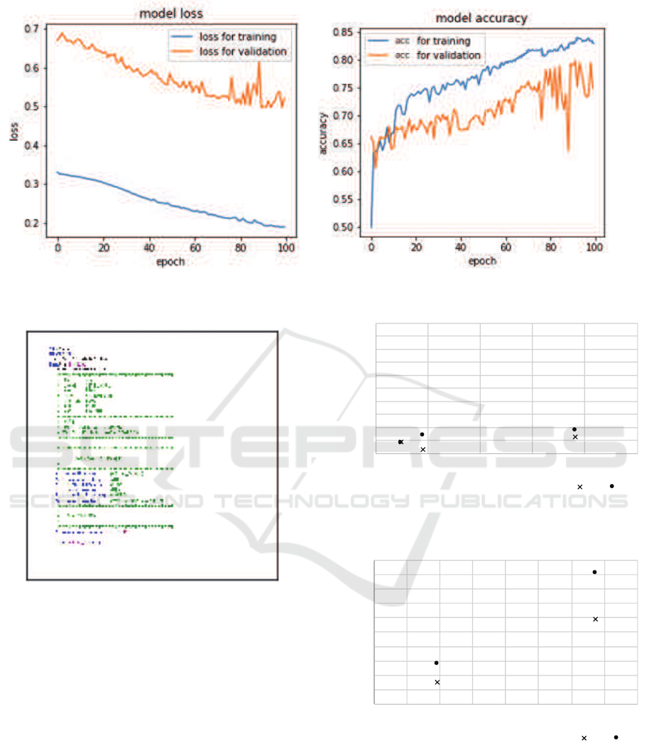
(a) Epoch vs. Loss (b) Epoch vs. Accuracy

Figure 3: Learning Process.

learn006_000001.jpg

Result: OK

[[0.41111973 0.5888802 ]]

Figure 4: An example of the results of an inference.

Figure 6 with the number of images on the x axis and

the number of labels of “BUG” on the y axis.

Corresponding to the results of the label “BUG,”

we examine precision, recall, and F measure. Table 2

shows the results.

In Table 2, Pg. is the serial number assigned to the

fragment of a program, while #Positive is the num-

ber of images that were inferred positively as the fault

prone programs, and thus labeled images as “BUG.”

#True is the number of images that were actually

modiﬁed fragments by ﬁxing bugs.

#TP. is the number of images in which defects were

detected or inferred correctly positive (true positive)

by the actual debugging process and inference.

There were however, bugs that could not be de-

100

0 50 100 150 200 250

Layer1

Layer2

The number of images of each program

Number of defects

Figure 5: A scatter plot of the number of images derived

from each program and the number of defects that were ac-

tually found in the program.

100

0 50 100 150 200 250 300 350 400

Layer1

Layer2

The number of images of each program

The number of defects

Figure 6: Scatter plot of the number of images and the num-

ber of inferred “BUG”s.

duced by the CNN. Table 3 shows the major defects

that could not be deduced.

Images that include SQL statements were success-

fully deduced as fault prone programs. In general,

syntax errors are detected by a compiler or a coding

tool, but it is hard to detect errors in SQL statements

Predicting Fault Proneness of Programs with CNN

325

Table 2: Precision, recall, and F measure.

Pg. #Posi- #True #TP. Preci- Re- F

tive sion call

a 8 9 6 0.75 0.67 0.71

b 14 3 2 0.14 0.67 0.24

c 28 15 7 0.25 0.47 0.33

d 18 13 3 0.17 0.23 0.19

e 91 59 41 0.45 0.69 0.55

Table 3: The major defects that could not be deduced.

Pg. Defects #cases

a Deletion of variables 1

a Deletion of program codes 2

b Correction of variables in the

condition of an IF statement

c Modiﬁcation of called functions 8

d Addition of program codes 4

d Modiﬁcation of program codes 3

d Deletion of program codes 3

e Addition and/or deletion of vari-

ables

e Addition of program codes 1

e Modiﬁcation of program codes 2

e Modiﬁcation of called functions 2

Table 4: Precision, Recall and F measure of the result of

interpretation of inference.

Pg. #Posi- #True #TP. Preci- Re- F

tive sion call

a 14 9 7 0.50 0.78 0.61

b 22 3 2 0.09 0.67 0.16

c 51 15 12 0.24 0.80 0.36

d 31 13 4 0.13 0.31 0.18

e 153 59 50 0.33 0.85 0.47

prior to the run time. The CNN was able to detect

such defects that were sometimes hard to ﬁnd. How-

ever, the inference of the CNN did not point out ac-

tual errors in the programs, but; the fault proneness

of each image. Therefore, after the CNN inference,

developers are expected to review the program frag-

ments that are inferred as fault prone programs.

There are problems we shall solve. When we com-

pared actual bugs with the inferred bugs, there were

multiple cases in which the image was labeled with

“BUG.”.

Table 4 shows precision, recall, and F measure

when we assumed that the CNN inferred the images

subsequent to accurate images.

Because the number of missing defects had de-

creased, the recall had increased, that said, the pre-

cision and F measure had decreased. In order to im-

prove precision, we should develop a method to cre-

ate images from programs with regard to the logic or

structure of the programs.

4 DISCUSSION

4.1 Possibility of Inference of Fault

Prone Programs

In this paper, we applied images of programs into

CNN in order to detect fault prone program frag-

ments. The machine learning system learned the re-

lationship between the fault and image based on the

supervised learning. After the machine learning was

completed, we analyzed the detected fault prone pro-

gram fragments and evaluated the machine learning

system.

4.1.1 Result of the Inference

Figure 5 and Figure 6 represent scatter plot with the

number of images of each program and the number

of actual/inferred faults. It means that the x-axis rep-

resents the size of each program and the y-axis rep-

resents their fault proneness. The scatter plot tells us

that there was a strong positive correlation between

the size of program and fault proneness. It is easy to

interpret this phenomena, since the number of faults,

as expected, increases according to the size of a pro-

gram. As shown in the diagrams, the number of in-

ferred faults was bigger than that of actual faults. This

is not a problem, because if the inference can point out

program fragments that need to be carefully reviewed,

we will be able to improve the quality of software.

4.1.2 Inference of Faults

As shown in Table 2, the recall of the inferred faults

was 0.68 at most. However, we now focus on faults

in Table 3 and pick up faults that were not inferred

by the machine learning system. The errors were as

follows;

• Mistakes of variable names in conditional state-

ments.

• Bugs in the addition and/or deletion of statements.

It must be difﬁcult for any CNN based systems to

detect such faults. These errors cannot be detected

through inferences based on images. Even so, the

CNN-BI system must still be useful. Bugs-prone pro-

gram fragments with SQL statements were detected

well.

The most important point of our research is that

we clarify the weak points of the CNN-BI system

when we apply the technique to improve the quality of

programs. We will be able to review the weak points

as well as the fault prone program fragments that are

successfully inferred by the CNN-BI system.

HAMT 2019 - Special Session on Human-centric Applications of Multi-agent Technologies

326

4.2 Quality of the Inference

The precision, recall, and F-measure are shown in Ta-

ble 4. Still now, we do not expect the CNN-BI sys-

tem to infer with high precision, but, with high recall.

It is important to gain greater recall than precision.

According to our application of the CNN inference,

recall is greater than precision for every project. In

contrast, if precision is greater than recall, we may

miss a lot of errors, and thus, and will not be able to

improve the quality of software.

4.2.1 Improve the Accuracy of Inference

In order to increase the accuracy of the inference, we

will collect a bigger training data set that will include

various kinds of defects other than SQL statements.

This is our future work.

4.2.2 Faults Inference with Images

Inferring defects in source codes by images of pro-

gram fragments are effective in detecting defects in

programs with SQL statements. The image of a pro-

gram with SQL statements may have a typical feature.

On the other hand, we found weakness in the CNN-

BI system. Addition and deletion of variables and/or

codes were not detected, since, these changes do not

seem to cause any changes in the data of supervised

learning.

The CNN-BI system’s recall could be 85%.

Though its precision was 33%, which is a result that

implies the review of programs still needs a lot of ef-

fort on the part of reviewers, we can conclude that the

inference with images for detecting fault prone pro-

gram fragments works well. The following issues re-

main to infer the fault prone fragments of programs:

• Improve the precision of the CNN-BI system.

In order to improve the precision, we need more

training data, and we may have to re-consider the

coloring rules. More or less colors may help the

CNN-BI system improve the precision of its in-

ference. When we convert a program fragment

to an image, for example, we can change the size

of characters. In our study, each program was di-

vided into several images based on the number of

lines of codes. There are other ways to divide each

program; e.g. structural blocks, etc.

• Improve the scalability and applicability of the

CNN-BI system.

In this study, we utilized program source codes

of a single project. We are not sure whether the

CNN-BI system is scalable and applicable to other

projects or not.

5 CONCLUSION

We have applied CNN with already trained data sets

in order to infer fault prone parts of programs by

transforming source codes to image data. The key of

our approach is the way to derive images from the

program source codes. We have taken advantages of

the strength of CNN to extract features from image

data.

We have demonstrated the effectiveness of our ap-

proach through the following processes.

• Analyze the inferred results as compared with the

ﬂaws that were actually found in target programs.

• Validate the result of inferred defects in the source

code.

According to the results, we have succeeded in in-

ferring fault prone parts of programs. Here are the

answers to the research questions.

• The CNN-BI system could extracted features of

fault proneness from images of programs. Even

though the inference is not perfect, we can use

our system to designate the focal points of pro-

gram reviews. The CNN-BI system is effective

to predetermine where we need to concentrate to

investigate programs.

• We have successfully identiﬁed some typical

ﬂaws in programs. We also found that some cat-

egories of problems are hard to ﬁnd with our ap-

proach.

• The accuracy of the inference acceptable was ac-

cepted in our study. We discussed the possible

ways to improve the accuracy of the inference.

In the experiments, we have applied CNN to a

small number of training data. In order to improve

the accuracy of the inference, we need to train the

CNN with a much larger collection of training data

(programs).

In our future work, we need to expand our ap-

proach to grasp a much larger set of defects, which

will contribute to the improvement of the quality of

software.

REFERENCES

Chidamber, S. R. and Kemerer, C. F. (1994). A metrics

suite for object oriented design. IEEE Transactions

on Software Engineering, 20(6):476–493.

Japkowicz, N. (2000). Learning from imbalanced data sets:

A comparison of various strategies. In AAAI Technical

Report WS-00-05. AAAI.

Predicting Fault Proneness of Programs with CNN

327

Kambayashi, Y. and Takimoto, M. (2005). Higher-order

mobile agents for controlling intelligent robots. Inter-

national Journal of Intelligent Information Technolo-

gies (IJIIT), 1(2):28–42.

Kondo, M., Mori, K., Mizuno, O., and Choi, E.-H. (2018).

Just-in-time defect prediction applying deep learning

to source code changes (in japanese). Journal of In-

formation Processing Systems, 59(4):1250–1261.

Le, Q. V., Ranzato, M., Monga, R., Devin, M., Chen, K.,

Corrado, G. S., Dean, J., and Ng, A. Y. (2012). Build-

ing high-level features using large scale unsupervised

learning. In Proc. of the 29th International Confer-

ence on Machine Learning, Edinburgh.

Lorenz, M. and Kidd, J. (1994). Object-Oriented Software

Metrics. Prentice-Hall.

Mayer, B. (2000). Object-Oriented Software Construction,

2nd ed. Prentice Hall.

McCabe, T. J. (1976). A complexity measure. IEEE Trans-

actions on Software Engineering, SE-2:308–320.

Morisaki, M. (2018). Deep learning use cases and their

points and tips : 6. review source code with AI. IPSJ

Magazine, 59(11):985–988.

Shehory, O. and Sturm, A., editors (2016). Agent-Oriented

Software Engineering: Reﬂections on Architectures,

Methodologies, Languages, and Frameworks (English

Edition). Springer.

Weiss, K., Khoshgoftaar, T. M., and Wang, D. (2016). A

survey of transfer learning. Journal of Big Data,

3(1):9.

Yang, X., Lo, D., Xia, X., Zhang, Y., and Sun, J. (2015).

Deep learning for just-in-time defect prediction. In

2015 IEEE International Conference on Software

Quality, Reliability and Security, pages 17–26.

Zimmermann, T., Premraj, R., and Zeller, A. (2007). Pre-

dicting defects for eclipse. In Third International

Workshop on Predictor Models in Software Engineer-

ing (PROMISE’07: ICSE Workshops 2007), pages 9–

15.

HAMT 2019 - Special Session on Human-centric Applications of Multi-agent Technologies

328