
Generalized Dirichlet Regression and other Compositional Models with
Application to Market-share Data Mining of Information Technology
Companies
Divya Ankam
a
and Nizar Bouguila
b
CIISE, Concordia University, Montreal, Canada
Keywords:
Compositional Data, Dirichlet Regression, Generalized Dirichlet, Market-shares, Financial Data Mining.
Abstract:
We explore the idea that market-shares of any given company have a linear relationship with the number of
times the company/product is searched for on the internet. This relationship is critical in deducing whether the
funds spent by a firm on advertisements have been fruitful in increasing the market-share of the company. To
deduce the expenditure on advertisement, we consider google-trends as a replacement resource. We propose a
novel regression algorithm, generalized Dirichlet regression, to solve the resulting problem with information
from three different information-technology fields: internet browsers, mobile phones and social networks.
Our algorithm is compared to Dirichlet regression and ordinary-least-squares regression with compositional
transformations. Our results show both the relationship between market-shares and google-trends, and the
efficiency of generalized Dirichlet regression model.
1 INTRODUCTION
Our aim is to predict the change in market-share
(Morais et al., 2018) (Tay and Mc Carthy, 1991) com-
position with respect to share-of-voice on social me-
dia. We assume it is directly proportional to the in-
vestment in marketing. We are making a strong as-
sumption that the google trends are a result of the
user’s search which were guided by advertisements
and people talking about the company/product. We
can thus deduce it to be directly proportional to the
money the company spends on advertising the prod-
uct (Cantner et al., 2012). The insider information
on the companies spendings on advertisements is not
readily available, though it would be a valuable piece
of information to have, it is confidential and the com-
panies are not obliged to disclose it. It could also give
the competitors an edge. Google-trends provides data
on ”interest over time” of the respective companies.
This could be a good measure of share-of-voice for
the company. This will be the independent predictor.
Market share (Moraisab et al., 2016) (Dussauge et al.,
2002) of company or similar data can be obtained as
a monthly statistic for few years. This will be propor-
tional data, assumed to follow a generalized Dirichlet
a
https://orcid.org/0000-0002-6898-4953
b
https://orcid.org/0000-0001-7224-7940
distribution (Fan and Bouguila, 2013b) (Bouguila and
Ziou, 2004b). This will be the prediction.
Mathematically compositional data (Aitchison,
1982) (Fan et al., 2013) are represented in a standard
simplex of the sample space given by,
S
D
= {x = [x
1
,x
2
,...,x
D
] ∈ R
D
} (1)
where x
i
> 0,i = 1, . . . , D and
∑
D
i=1
x
i
= k ; x is a D-
dimensional vector of features representing a given
object (e.g. document, image, video, etc.) and k is
a constant.
Regression problems based on compositional data
can be categorized into 2 groups. In the first group
the dependant variable is compositional (Ankam and
Bouguila, 2018), such problems have been solved
by using Aitchison’s geometric transformations. In
the second group the response variables are composi-
tional, with either same or different predictors. The
latter type of problems is more complex and this is
what we have tackled in this paper. So far, Dirichlet
regression (Maier, 2014) (Bouguila and Ziou, 2004a)
has been the best approach in the industry to define
compositional regression problems where the depen-
dent variables are compositional.
In this paper, we develop generalized Dirichlet
(GD) regression, where the dependent variables fol-
low a generalized Dirichlet distribution (Zhang et al.,
2017) (Bouguila and Ziou, 2006). With double the
158
Ankam, D. and Bouguila, N.
Generalized Dirichlet Regression and other Compositional Models with Application to Market-share Data Mining of Information Technology Companies.
DOI: 10.5220/0007708201580166
In Proceedings of the 21st International Conference on Enterprise Information Systems (ICEIS 2019), pages 158-166
ISBN: 978-989-758-372-8
Copyright
c
2019 by SCITEPRESS – Science and Technology Publications, Lda. All rights reserved

number of parameters to estimate in comparison with
the Dirichlet, GD is more versatile and gives space to
model a flexible line of fit. We show how data fit-
ting can be done by using a geometric transformation
that reduces the generalized Dirichlet into a product
of Beta distributions.
The rest of the paper describes the main crux of
our research, it will answer the pinching question,
will the Google trends be able to predict the rise and
fall of shares in any given field? To demonstrate the
same, we have chosen the following three interesting
quintessential markets of the modern world, related
to technology and communication, mobile vendors in
Canada, social network sites in India and what is the
most used browser in the world! Let’s explore this
case and discuss how successful is Google-trends in
predicting the trends of the share markets. Section 2
describes the machine learning algorithms employed
for the research. Section 2.3.3 explains our contribu-
tion in devising the GD regression algorithm. Section
3 gives the background for experimental set-up. Sec-
tion 4 shows our results and analysis. We conclude
with Section 5.
2 MACHINE LEARNING
TECHNIQUES
In this section we discuss the various ML algorithms
used in our research. They are explained in the in-
creasing order of computational complexity. Start-
ing from ordinary least squares with a combination of
transformations like clr and ilr. After which we de-
scribe Beta regression, Dirichlet regression and gen-
eralised Dirichlet regression.
2.1 OLS - Ordinary Least Squares
Regression
Ordinary least squares (OLS) regression is a case of
generalized linear modelling algorithm. It employs
linear least squares method for estimating a single re-
sponse variable. It could be multivariate of single in-
dependant variable x, to predict the response (Fox and
Monette, 2002). Principle of least squares minimizes
the sum of squares of the differences between the ac-
tual response y, in the given data and prediction of the
linear function (Hutcheson, 2011). If we consider a
linear system of variables, with n data points:
n
∑
j=1
X
i j
β
j
= y
i
,(i = 1,2,...,m) (2)
here β is the regression co-efficient
Xβ = y (3)
where
X =
X
11
X
12
··· X
1n
X
21
X
22
··· X
2n
.
.
.
.
.
.
.
.
.
.
.
.
X
m1
X
m2
··· X
mn
,
β =
β
1
β
2
.
.
.
β
n
,y =
y
1
y
2
.
.
.
y
m
(4)
Such a system usually has no arithmetic solution,
rather the aim is to find the best coefficients β which
better fit the equations, to solve the quadratic mini-
mization problem
ˆ
β = argmin
β
S(β) (5)
where the objective function S is given by
S(β) =
∑
m
i=1
y
i
−
∑
n
j=1
X
i j
β
j
2
= ky −Xβk
2
(6)
Finally,
ˆ
β is the coefficient vector of the least-squares
hyperplane, expressed as a product of Gramiam ma-
trix of X and moment matrix of regressors:
ˆ
β =
X
T
X
−1
X
T
y (7)
2.2 Aitchison Transformations
In the share market case, both dependent and in-
dependent variables are compositional. Hence both
are transformed to the Aitchison plane by applying
the transformations explained below. Then, they are
fed to ordinary least squares regression algorithm
(ols). The resultant matrix is transformed back to
Euclidean plane by applying an inverse transform.
Then, the actual and predicted values are compared
against the selection criteria explained in section 3.2.
We discuss two Aitchison transformations (Aitchison,
1982), CLR (centred log ratio transform) and ILR
(Isometric log ratio transform). These are widely used
in the case of compositional data.
2.2.1 Centered Log Ratio (CLR) + OLS
CLR is defined as:
y = (y
1
,...,y
D
)
0
=
ln
x
1
D
q
∏
D
i=1
x
i
,...,ln
x
D
D
q
∏
D
i=1
x
i
!
0
(8)
Generalized Dirichlet Regression and other Compositional Models with Application to Market-share Data Mining of Information
Technology Companies
159

CLR can also be represented as follows
y = {y
i
}
i=1,...,D
=
n
ln
x
i
g(x)
o
i=1,...,D
(9)
g(x) =
D
∏
j=1
x
j
1/D
(10)
Here g(x) is the geometric mean of the composition.
Resulting in D variables, each representing one com-
ponent of the original compositional part. Individual
contribution of each part is easily interpretable. Sub-
compositional incoherence and generation of singular
matrix are the drawbacks of CLR. Singular data is in-
compatible with most of the present statistical analy-
sis methods. This can be overcame by ILR transfor-
mation.
2.2.2 Isometric Log Ratio (ILR) + OLS
ILR is defined as:
z
i
=
r
D − i
D − i + 1
ln
x
i
D−i
q
∏
D
j=i+1
x
j
,i = 1,...,D − 1
(11)
This results in D − 1 coordinates in a chosen or-
thonormal basis. It represents only the ratios between
the components. ILR can also be represented in terms
of CLR as
z = Hy (12)
Where H is the Helmert sub- matrix, obtained by re-
moving the first row of Helmert matrix (Lancaster,
1965). H is a popular orthonormal basis. ILR is ap-
plied on data matrix X, subsequent ILR co-ordinates Z
are fed into the OLS algorithm in section 2.1. The re-
gression coefficient matrix thus obtained, using equa-
tion (3) is γ, has (D − 1) x n dimensions. When sub-
stituted in equation above, the predictor variables Y
are obtained.
2.3 Distributions-based Regression
2.3.1 Beta Regression
Assuming the response data is Beta distributed (Bayes
et al., 2012), The authors in (Ferrari and Cribari-Neto,
2004) have proposed a regression model with mean
and dispersion parameters of the distribution. In con-
trary to the transformed response of a linear regres-
sion, Beta regression’s parameters are deduced using
maximum likelihood estimation. The Beta density
function is given as follows:
Y ∼ B(p,q), f (y; p, q) =
Γ(p + q)
Γ(p)Γ(q)
y
p−1
(1 − y)
q−1
(13)
Maximum likelihood estimation is performed to de-
duce the values of p and q. The closed form solution
to this equation is given in (Ferrari and Cribari-Neto,
2004). The partial derivatives of log of Beta distribu-
tion with respect to p and q are given by
∂log f (y; p,q)
∂p
= ψ(p + q) − ψ(p) + log y (14)
∂log f (y; p,q)
∂q
= ψ(p + q) −ψ(q) + log(1 − y) (15)
Where ψ(.) is the digamma function defined as
Γ(x) =
Z
∞
0
t
x−1
exp(−t)dt (16)
The expected score equals zero, it can be re-written
as:
E[logY ] = ψ(p) − ψ(p + q) (17)
E[log(1 −Y )] = ψ(q)− ψ(p + q) (18)
The distribution of response variable Y
i
is B (p
i
,q
i
)
where p
i
and q
i
are, for each i, described by sets of
explanatory variables (x
1
,...,x
m
) and (v
1
,...,v
M
) as
p
i
= g(β
1
x
1i
+ ··· + β
m
x
mi
) (19)
q
i
= h(γ
1
v
1i
+ ··· + γ
M
v
Mi
) (20)
Here g and h are link functions. The above equations
can be substituted in the log likelihood equation of
Beta distribution
`(θ) =
n
∑
i=1
logΓ(p
i
+ q
i
) −
n
∑
i=1
logΓ(p
i
) −
n
∑
i=1
logΓ(q
i
)
+
n
∑
i=1
p
i
logy
i
+
n
∑
i=1
q
i
log(1 − y
i
)
(21)
Whose first order derivatives are given by
∂`
∂β
r
=
n
∑
i=1
g
0
i
x
ri
[ψ(p
i
+ q
i
) − ψ (p
i
) + log y
i
]
∂`
∂γ
R
=
n
∑
i=1
h
0
i
v
Ri
[ψ(p
i
+ q
i
) − ψ (q
i
) + log (1 − y
i
)]
(22)
Maximum likelihood estimation of β and γ are ob-
tained by solving the above equations, equating to
zero. Thus, the regression parameters are obtained.
They can be multivariate or univariate, depending on
the application. It has to be noted that, in the case
of compositional data, where the predicted values are
more than one, the Beta regression needs to be ex-
tended to accommodate the prediction of multiple de-
pendant variables. This is explored in the further two
sections, Dirichlet regression and generalized Dirich-
let regression.
ICEIS 2019 - 21st International Conference on Enterprise Information Systems
160

2.3.2 Dirichlet Regression
Marco J Maier has proposed Dirichlet regression
(Maier, 2014) (Hijazi and Jernigan, 2009), which as-
sumes the dependent variables are compositional and
follow a Dirichlet distribution. He has deduced a
framework similar to general linear models for regres-
sion of Dirichlet distributed data. Dirichlet distribu-
tion is a generalized form of Beta distribution (Fan
and Bouguila, 2013a), defined in equation 23. Also
known as common parametrization.
D(y|α) =
1
B(α)
C
∏
c=1
y
(a
c
−1)
c
(23)
where B(α) =
C
∏
c−1
Γ(α
c
)/Γ
C
∑
c−1
α
c
!
(24)
and Γ(x) =
Z
∞
0
t
x−1
exp(−t)dt (25)
Alternately, Dirichlet distribution can also be repre-
sented as a function of mean µ and variance φ as in
equation 26, called alternate parametrization.
f (y|µ,φ) =
1
B(µφ)
C
∏
c=1
y
(µ
c
φ−1)
c
(26)
The full log-likelihood of the commonly parametrized
model is defined below
`
c
(y|α) = log Γ
C
∑
c=1
α
c
!
−
C
∑
c=1
logΓ (α
c
) +
C
∑
c=1
(α
c
− 1)log (y
c
)
(27)
The crucial part of converting a Dirichlet distribution
to a Dirichlet regression problem, lies in the link be-
tween the Dirichlet parameters (α) and the regression
parameters (β). The link function g(.) is selected as a
log(.) function, defined as
g(α
c
) = η
c
= X
[c]
β
[c]
(28)
The first order derivative of the log-likelihood:
∂`
c
∂β
[d]
m
= x
[c]
m
α
[d]
"
log
y
[d]
− ψ
α
[d]
+ ψ
C
∑
c=1
α
[c]
!#
(29)
The second order derivatives of the log-likelihood
with respect to βs on the same and different variables
are given below. The Hessian matrix of the same can
be obtained from (Maier, 2014).
∂
2
`
c
∂β
[d]
m
∂β
[d]
n
= x
[d]
m
x
[d]
n
α
[d]
(
log(y
d
) + ψ
C
∑
c=1
α
c
!
− K
)
(30)
K = ψ(α
d
) − α
d
"
ψ
1
C
∑
c=1
α
c
!
− ψ
1
(α
d
)
#
(31)
∂
2
`
c
∂β
[d]
m
∂β
[e]
n
= x
[d]
m
x
[e]
n
α
d
α
e
ψ
1
C
∑
c=1
α
c
!
(32)
Caution is to be taken to resist the urge to calculate α
of the Dirichlet distributed dependent variables. As
this is not the desired output, We are more interested
in calculating the regression parameters β, which
will be found only after relating it to α in the link
function. The maximum log-likelihood estimation
(MLE) of Dirichlet regression is different from that
of Dirichlet distribution MLE.
2.3.3 Generalized Dirichlet (GD) Regression
We now propose generalized Dirichlet regression to
solve the compositional regression problems of inter-
est. This distribution has double the number of pa-
rameters to estimate compared to Dirichlet distribu-
tion. This gives it more degrees of freedom to fit the
data in a better way. It’s probability density function
is as follows
c
n
∏
i=1
x
a
i
−1
i
1 −
i
∑
k=1
x
k
!
b
i
−1
(33)
To evaluate the normalizing constant c, we integrate
sequentially over x
n
,x
n−1
,...,x
2
,x
1
, where n is the
number of components of x.
c =
n
∏
i=1
Γ(1 +
∑
n
k=i
(a
k
+ b
k
− 1))
Γ(a
i
)Γ
b
i
+
∑
n
k=i+1
(a
k
+ b
k
− 1)
(34)
In an n dimensional GD distributed data, there are
2n variables to estimate. There would be 2n log-
likelihood equations to solve simultaneously. (Chang
et al., 2010) demonstrate that GD can be transformed
to n Beta distributions. Suppose (X
1
,...,X
n
) ∼
GD(a
1
,...,a
n
;b
1
,...,b
n
) Where Zi = Zi...Zn are n
mutually independent Beta distributed variables
Z
i
∼ B (a
i
,b
i
+(
n
∑
k=i+1
(b
k
+ a
k
− 1)),i = 1,...,n (35)
(X
1
,...,X
n
) ,
Z
1
,Z
2
(1 − Z
1
),...,Z
n
n−1
∏
i=1
(1 − Z
i
)
!
(36)
It follows that the problem can be reduced to n-
likelihood equations in pairs.
Z
i
= X
i
/
1 −
i−1
∑
j=1
X
j
!
∼ B(a
i
,c
i
) (37)
where i = 1,..., n for a random sample
(X
1 j
,...,X
n j
), j = 1, . . . , N, from X
1
,...,X
n
the
Generalized Dirichlet Regression and other Compositional Models with Application to Market-share Data Mining of Information
Technology Companies
161

corresponding log-likelihood function can be
expressed as follows:
N
∏
l=1
n
∏
i=1
Γ(a
i
+ c
i
)
Γ(a
i
)Γ (c
i
)
x
il
1 −
∑
i−1
j=1
x
jl
!
a
i
−1
∑
i
j=1
x
jl
1 −
∑
i−1
j=1
x
jl
!
c
i
−1
(38)
The first order derivatives of MLE are n pairs, where
i = 1,...,n is below:
0 =
∂logL
∂a
i
= ψ(a
i
)−ψ(a
i
+ c
i
)−
1
N
N
∑
l=1
logx
il
(39)
0 =
∂logL
∂c
i
= ψ(c
i
) − ψ (a
i
+ c
i
) −
1
N
N
∑
l=1
log(1 − x
il
)
(40)
Since a Dirichlet MLE has been transformed to n
Beta MLE, we will follow the steps in section 2.3.1 to
convert the Beta distribution to Beta regression esti-
mates using link function. Various link functions can
be used to relate the dependent variables to indepen-
dent variable, for example, log-link, logit-link, probit,
log-log link.
There is no closed form solutions for the above
equations. Newton-Raphson iteration is employed to
arrive at the solution in maximum likelihood estima-
tion. The initial values are obtained from method of
moments estimates. The estimated values of regres-
sion are normalised to equate to 1 as the expectation
is compositional data.
3 EXPERIMENTAL SET-UP
3.1 k-fold Cross Validation
Our aim is to create a replica of the underlying model
generating the data. The approach we follow is to
work backwards from the collected data. In the pro-
cess, there is a danger of over-fitting/under-fitting the
data. Which means, the model is created specifically
around the given data. Any newly generated data,
even though coming from the same source, will not
be described with this model. To overcome this is-
sue, we have used the method of k-fold cross valida-
tion (Watt et al., 2016). It is a systematic hold out
method, where the data is splitted into k parts. over a
loop of k times, each part is held out for testing and
the model is trained over the remaining data (total-kth
part). This way k different models are created, and the
features are averaged over the k models. This gives
equal opportunity for the data being represented fully
compared to randomized hold-out cross validation.
The k-fold algorithm is used to compute the av-
erage of evaluation measures, and it is called 1000
times to average out the measures over the different
partitions. Thus, each dataset is modelled 1000*10
times, that is 10,000 times for a 10-fold cross vali-
dation. This is the most computationally expensive
component of the regression problem we are solving.
Algorithm 1: k-fold cross-validation pseudo-code.
Input Dataset, number of folds k,
Split the data into k equally sized (rounded to
integer) folds
1: procedure K-FOLD-REGRESSION
2: for <s = 1:k> do
3: Train a model on sth fold’s training set
4: Test the model on sth fold’s test set
5: Compute corresponding evaluation measures
6: Compute average of evaluation measures of
all k sets
3.2 Evaluation Measures
The goodness of fit of the regression models need to
be measurable. This helps us decide which model
is able to describe the data best. Since we are deal-
ing with compositional data, the regular measures of
regression need to be modified accordingly, There
are various measures explained in (Hijazi, 2006).
The efficacy of the learned models is compared with
these three parameters, sum of square of residuals, R-
squared measure based on total variability and KL di-
vergence.
3.2.1 R-squared Measure based on Total
Variability (R2T)
The term total variability based R square measure
was coined by Aitchison in the log ratio analy-
sis[Aitchison 1986]. It is defined as the ratio of total
variance in the predicted values to the total variance
in the actual values.
R
2
T
= totvar(
b
x)/totvar(x) (41)
T(x) = [τ
i j
] =
var
log(x
i
/x
j
)
(42)
totvar(x) =
1
2d
∑
T(x) (43)
3.2.2 Residual Sum of Squares (RSS)
Residual sum of squares (RSS) (Draper and Smith,
2014) is defined as the square of the difference be-
tween the predicted and actual values for each point
ICEIS 2019 - 21st International Conference on Enterprise Information Systems
162

in test set. In the compositional case, the sum of each
component’s RSS is summed up.
RSS =
n
∑
i=1
(y
i
−
b
y
i
)
2
(44)
3.2.3 Kullback-Leibler Divergence (KL)
KL divergence is the sum of ratio of the logarithm of
actual values o fitted values, weighed by the actual,
over each data point(Kullback and Leibler, 1951).
Minimum KL divergence is desired as it deduces
maximum likelihood (Haaf et al., 2014).
KL(S,
b
S) =
T
∑
t=1
D
∑
j=1
log
S
jt
b
S
jt
!
S
jt
(45)
KL divergence adapted to compositional data is de-
fined as follows (Martin-Fernandez et al., 1999):
KLC(S,
b
S) =
D
2
KL
0
D
,S
b
S
+ KL
0
D
,
b
S S
(46)
=
D
2
T
∑
t=1
log
S
t
/
b
S
t
·
b
S
t
/S
t
(47)
4 DATASETS AND RESULTS
In order to assess the usefulness of the regression
models,we have investigated 2 real-life data sets fol-
lowed by 3 different applications based on data col-
lected from real-life sources. The market shares data
are obtained from global-stats
1
website, the relation
we are trying to observe is the company’s market-
share to their trends in google-searches
2
, which is a
good measure of the company’s investment in adver-
tising.
4.1 Real Data
4.1.1 Arctic Lake Soil Compositions Dataset
We discuss Arctic lake data set, which shows how the
composition of ground soil comprising of silt, sand
and clay is altered as the depth of lake increases. This
is a famous dataset used by Aitchison to investigate
many transformations. It has been quoted in stud-
ies, like zero value substitution (Tsagris and Stewart,
2018) (Tsagris, 2015) and robustness checks (Tsagris,
2015). There are 39 data points with three compo-
nents. The distribution of the data points is shown in
1
http://gs.statcounter.com
2
https://trends.google.com/trends/
ternary diagram, Figure 1. Unlike most regression
problems, with a single response variable and multi-
ple independent variables, the Arctic lake data is dif-
ferent. It has a single independent variable (x) and
three different response variables, whose sum adds up
to unity. It is the compositions that we are predicting.
We could use a variety of arithmetic transformations
of x, like log(x), x
2
, x + x
2
. Table 1 shows the regres-
sion measures of the different regression algorithms
explained in the above sections. GD regression has
least residual sum of squares, which represents a good
fit. Dirichlet regression is the best in this case, given
R2T and KL divergence measures.
4.1.2 Glass Composition Dataset
Another dataset containing more number of composi-
tions is the forensic glass dataset (Tsagris and Stew-
art, 2018). It has 8 components and 214 observations.
They are are all dependant on a single parameter, the
refractive index (RI) of glass. The aim is to map how
the refractive index of glass can alter the composition
of glass, the minerals in it, like Aluminium, magne-
sium to name a few. The regression should ideally
appear the other way round, the RI is determined by
the composition. But, we are doing the reverse pro-
cess to see if we can find the required composition to
be able to manufacture/recreate the intended RI. As
per the results in Table 2, least SSR is by GD regres-
sion algorithm. Better KL divergence is shown by the
classical OLS methods, this could be due to the un-
equal distribution of metals in the glass. Some metals
like Silicon and Sodium have high compositions com-
pared to the rest.
4.2 Application - Market Shares for
Information Technology Companies
For future researchers to be able to reproduce our
work, we have chosen the public platform of google-
trends (Choi and Varian, 2012) (Vosen and Schmidt,
2011). It gives us a very good idea on how the data
search has spiked over the given time range, which is
of prime importance. Here have been a couple of ex-
periments done to see if any lag in trends and share is
observed. Trends seems to be more real time and the
data seemed to be more relevant to the current mar-
ket share. A lag of two months is observed between
the trends and market shares. The companies invest-
ment on advertisements seem to have been fruitful a
couple of months later in getting the google clicks
and thus for it to show effect on the market share.
We would further like to explain how the shares have
changed over the time, any interesting patterns are ex-
Generalized Dirichlet Regression and other Compositional Models with Application to Market-share Data Mining of Information
Technology Companies
163
plained. It is to be noted that google-trends (Carri
`
ere-
Swallow and Labb
´
e, 2013) only supports comparison
of 5 key-words at a time. To support more searches,
we will compare the term with a standard term such as
”photo” to get a relative measure of frequency. This
process is done with all the variables, then put to-
gether and normalized.
4.2.1 Browser Market Shares - Worldwide
It is interesting to note, in 2009, Internet-Explorer
(64.97%) and Firefox (26.85%) were leading the mar-
ket, and today they are mere 3-5% share holders in
the world-wide browser markets. This owes to the in-
troduction of new browser by Google, Chrome and
Apple’s Safari. The major market shares in internet
browsers is held by Chrome (51.5%) followed by Sa-
fari (15.13%) in 2018. We have collected monthly
from 2009 January to 2018 September, with n = 118
data points, with D = 6 components, including UC
browser and Opera. The ternary diagrams of 3 sets
of browsers are given in Figures 2, 3, 4 and 5. This
shows how the compositions have changed over the
course of 10 years. They clearly follow a linear pat-
tern. Table 3 has the results of the experiment. It
is observed that GD regression shows close to unity
R2T, and least KL divergence (0.23). Dirichlet re-
gression has slightly better RSS (0.03) than GD re-
gression (0.09). The arithmetic transforms combined
with OLS with less computational complexity, take
lesser time to execute, with acceptable results.
4.2.2 Mobile Seller Market Shares in Canada
The Canadian mobile market was ruled by Apple
(88.97%) in the year 2010. It is now sharing space
with Samsung (25.14%) in 2018. We have included
LG, Huawei, Google and Motorola in the study. With
D = 6 and n = 95, we have the independent variables
obtained from Google-trends, individually for each
company, the trends are in accordance with the share
market patterns. Table 4 describes the results. Look-
ing at the measures, we can say that google trends has
been a good measure of predicting the shares, with
the regression fits of RSS close to zero. The general-
ized Dirichlet regression performed well compared to
other methods.
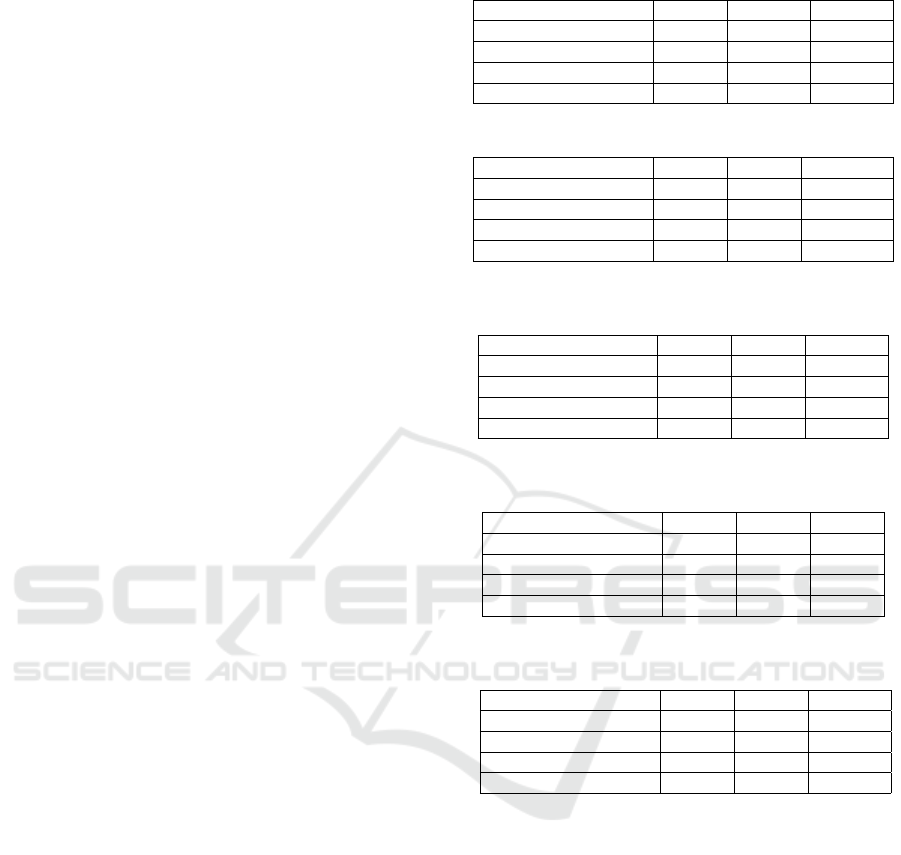
Table 1: Regression measures of Arctic lake sediments data.
Methods\Measures SSR R2T KL
CLR + OLS 3.3287 11.0777 25.4432
ILR + OLS 3.3183 11.8528 25.3671
Dirichlet regression 0.8193 6.2170 15.9382
Generalized Dirichlet 0.5415 8.9557 17.9848
Table 2: Regression measures of forensic glass data.
Methods\Measures SSR R2T KL
CLR + OLS 9.4718 0.0126 216.8152
ILR + OLS 9.4577 0.0129 217.3527
Dirichlet regression 0.0186 0.0023 333.3006
Generalized Dirichlet 0.0145 0.0015 336.3690
Table 3: Regression measures of world-wide browser
shares.
Methods\Measures SSR R2T KL
CLR + OLS 4.1566 0.9075 0.7468
ILR + OLS 6.2981 0.0386 11.4344
Dirichlet regression 0.0279 1.0533 0.2290
Generalized Dirichlet 0.0840 0.8230 0.8385
Table 4: Regression measures of mobile vendor shares in
Canada.
Methods\Measures SSR R2T KL
CLR + OLS 4.9768 5.6769 9.6099
ILR + OLS 4.9934 0.3337 9.1590
Dirichlet regression 0.0004 0.9443 0.0044
Generalized Dirichlet 0.0100 0.2747 0.1194
Table 5: Regression measures of Social Media Shares in
India.
Methods\Measures SSR R2T KL
CLR + OLS 5.0926 0.0419 11.3324
ILR + OLS 5.1004 0.0395 11.4662
Dirichlet regression 0.0720 0.0741 11.5216
Generalized Dirichlet 0.6679 0.1262 21.2748
4.2.3 Social Networks Market Shares in India
Facebook is the most followed social networking site
in India. It has been growing popularity from 52.3%
in 2010 to 86.56% in October 2018. Many companies
have mushroomed in this space but Youtube has sus-
tained it’s second place with 10% and it saw it’s peak
with 25% in 2012. Twitter had a good 7% share in
2013, but now it has a mere 1% share. Results have
been recorded in Table 5. Dirichlet regression seems
to fit the data better than GD regression, with slight
variation in the measures.
ICEIS 2019 - 21st International Conference on Enterprise Information Systems
164
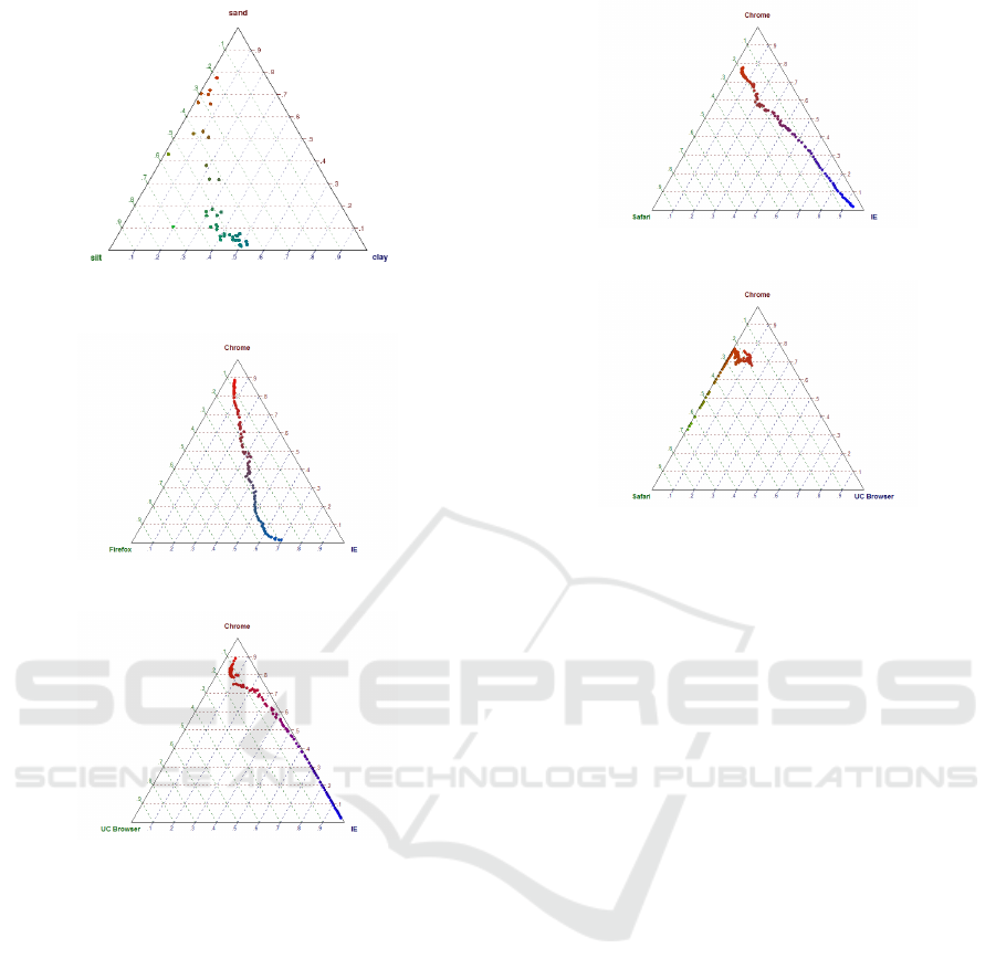
Figure 1: Arctic Lake.
Figure 2: Browser shares: Chrome, IE, Firefox.
Figure 3: Browser shares: Chrome, IE, UC.
5 CONCLUSION
We have introduced an implementation of general-
ized Dirichlet regression that extends Beta regres-
sion for compositional, multiple response variables.
An application in share-market analysis demonstrates
the modelling capabilities of this solution. Vari-
ous compositional regression models have been dis-
cussed, and their results compared. The question, ”Is
google-trends a good predictor of the share market
dynamics?” is answered with three real-world exam-
ples. Google trends seem to capture the share-market
trends well. The distribution-based regression algo-
rithms fared better than transformations-based regres-
sion. Though the trade-off is the use of more compu-
tationally complex calculations.
Additionally, we suggest future work should ex-
plore new choices of starting values for the maxi-
Figure 4: Browser shares: Chrome, Safari, IE.
Figure 5: Browser shares: Chrome, UC, Safari.
mum likelihood estimation of generalized Dirichlet
regression and their corresponding sensitivity stud-
ies for these choices. A more robust system with
less sensitivity to the estimation of regression coef-
ficients could be developed, with the use of mixture
models (Bouguila and Ziou, 2012) in Dirichlet regres-
sion. This work could be applied in the fields of image
recognition (Boutemedjet et al., 2007) and intrusion
detection (Fan et al., 2011).
ACKNOWLEDGEMENTS
The completion of this work was made possible
thanks to NSERC and Concordia University research
chair.
REFERENCES
Aitchison, J. (1982). The statistical analysis of composi-
tional data. Journal of the Royal Statistical Society.
Series B (Methodological), pages 139–177.
Ankam, D. and Bouguila, N. (2018). Compositional data
analysis with pls-da and security applications. In 2018
IEEE International Conference on Information Reuse
and Integration (IRI), pages 338–345. IEEE.
Bayes, C. L., Baz
´
an, J. L., Garc
´
ıa, C., et al. (2012). A new
robust regression model for proportions. Bayesian
Analysis, 7(4):841–866.
Bouguila, N. and Ziou, D. (2004a). Dirichlet-based prob-
ability model applied to human skin detection [im-
age skin detection]. In 2004 IEEE International Con-
Generalized Dirichlet Regression and other Compositional Models with Application to Market-share Data Mining of Information
Technology Companies
165

ference on Acoustics, Speech, and Signal Processing,
ICASSP 2004, Montreal, Quebec, Canada, May 17-
21, 2004, pages 521–524.
Bouguila, N. and Ziou, D. (2004b). A powerful finite
mixture model based on the generalized dirichlet dis-
tribution: Unsupervised learning and applications.
In 17th International Conference on Pattern Recog-
nition, ICPR 2004, Cambridge, UK, August 23-26,
2004., pages 280–283.
Bouguila, N. and Ziou, D. (2006). A hybrid SEM algorithm
for high-dimensional unsupervised learning using a fi-
nite generalized dirichlet mixture. IEEE Trans. Image
Processing, 15(9):2657–2668.
Bouguila, N. and Ziou, D. (2012). A countably infinite mix-
ture model for clustering and feature selection. Knowl.
Inf. Syst., 33(2):351–370.
Boutemedjet, S., Ziou, D., and Bouguila, N. (2007). Unsu-
pervised feature selection for accurate recommenda-
tion of high-dimensional image data. In Advances in
Neural Information Processing Systems 20, Proceed-
ings of the Twenty-First Annual Conference on Neural
Information Processing Systems, Vancouver, British
Columbia, Canada, December 3-6, 2007, pages 177–
184.
Cantner, U., Kr
¨
uger, J. J., and S
¨
ollner, R. (2012). Product
quality, product price, and share dynamics in the ger-
man compact car market. Industrial and Corporate
Change, 21(5):1085–1115.
Carri
`
ere-Swallow, Y. and Labb
´
e, F. (2013). Nowcasting
with google trends in an emerging market. Journal
of Forecasting, 32(4):289–298.
Chang, W.-Y., Gupta, R. D., and Richards, D. S. P. (2010).
Structural properties of the generalized dirichlet dis-
tributions. Contemp. Math, 516:109–124.
Choi, H. and Varian, H. (2012). Predicting the present with
google trends. Economic Record, 88:2–9.
Draper, N. R. and Smith, H. (2014). Applied regression
analysis, volume 326. John Wiley & Sons.
Dussauge, P., Garrette, B., Mitchell, W., et al. (2002). The
market-share impact of inter-partner learning in al-
liances: evidence from the global auto industry. Co-
operative strategies and alliances, pages 707–727.
Fan, W. and Bouguila, N. (2013a). Online learning of
a dirichlet process mixture of beta-liouville distribu-
tions via variational inference. IEEE transactions on
neural networks and learning systems, 24(11):1850–
1862.
Fan, W. and Bouguila, N. (2013b). Variational learning of a
dirichlet process of generalized dirichlet distributions
for simultaneous clustering and feature selection. Pat-
tern Recognition, 46(10):2754–2769.
Fan, W., Bouguila, N., and Ziou, D. (2011). Unsupervised
anomaly intrusion detection via localized bayesian
feature selection. In 11th IEEE International Confer-
ence on Data Mining, ICDM 2011, Vancouver, BC,
Canada, December 11-14, 2011, pages 1032–1037.
Fan, W., Bouguila, N., and Ziou, D. (2013). Unsuper-
vised hybrid feature extraction selection for high-
dimensional non-gaussian data clustering with vari-
ational inference. IEEE Trans. Knowl. Data Eng.,
25(7):1670–1685.
Ferrari, S. and Cribari-Neto, F. (2004). Beta regression for
modelling rates and proportions. Journal of Applied
Statistics, 31(7):799–815.
Fox, J. and Monette, G. (2002). An R and S-Plus companion
to applied regression. Sage.
Haaf, C. G., Michalek, J. J., Morrow, W. R., and Liu, Y.
(2014). Sensitivity of vehicle market share predictions
to discrete choice model specification. Journal of Me-
chanical Design, 136(12):121402.
Hijazi, R. H. (2006). Residuals and diagnostics in dirichlet
regression. ASA Proceedings of the General Method-
ology Section, pages 1190–1196.
Hijazi, R. H. and Jernigan, R. W. (2009). Modelling compo-
sitional data using dirichlet regression models. Jour-
nal of Applied Probability & Statistics, 4(1):77–91.
Hutcheson, G. D. (2011). Ordinary least-squares regres-
sion. The SAGE Dictionary of Quantitative Manage-
ment Research, pages 224–228.
Kullback, S. and Leibler, R. A. (1951). On information
and sufficiency. The annals of mathematical statistics,
22(1):79–86.
Lancaster, H. (1965). The helmert matrices. The American
Mathematical Monthly, 72(1):4–12.
Maier, M. J. (2014). Dirichletreg: Dirichlet regression for
compositional data in r.
Martin-Fernandez, J. A., Bren, M., Barcelo-Vidal, C., and
Pawlowsky Glahn, V. (1999). A measure of differ-
ence for compositional data based on measures of di-
vergence. Proceedings of IAMG, 99:211–216.
Morais, J., Thomas-Agnan, C., and Simioni, M. (2018).
Using compositional and dirichlet models for mar-
ket share regression. Journal of Applied Statistics,
45(9):1670–1689.
Moraisab, J., Thomas-Agnana, C., and Simionic, M.
(2016). A tour of regression models for explaining
shares.
Tay, R. S. and Mc Carthy, P. S. (1991). Demand ori-
ented policies for improving market share in the us
automobile industry. International Journal of Trans-
port Economics/Rivista internazionale di economia
dei trasporti, pages 151–166.
Tsagris, M. (2015). Regression analysis with composi-
tional data containing zero values. arXiv preprint
arXiv:1508.01913.
Tsagris, M. and Stewart, C. (2018). A dirichlet re-
gression model for compositional data with zeros.
Lobachevskii Journal of Mathematics, 39(3):398–
412.
Vosen, S. and Schmidt, T. (2011). Forecasting private con-
sumption: survey-based indicators vs. google trends.
Journal of Forecasting, 30(6):565–578.
Watt, J., Borhani, R., and Katsaggelos, A. K. (2016). Ma-
chine Learning Refined: Foundations, Algorithms,
and Applications. Cambridge University Press.
Zhang, Y., Zhou, H., Zhou, J., and Sun, W. (2017). Regres-
sion models for multivariate count data. Journal of
Computational and Graphical Statistics, 26(1):1–13.
ICEIS 2019 - 21st International Conference on Enterprise Information Systems
166
