
Accuracy Assessment of a Photogrammetric UAV Block by using
Different Software and Adopting Diverse Processing Strategies
Vittorio Casella
1
, Filiberto Chiabrando
2
, Marica Franzini
1
and Ambrogio Maria Manzino
3
1
Department of Civil Engineering and Architecture, University of Pavia, Pavia, Italy
2
Department of Architecture and Design, Polytechnic of Turin, Turin, Italy
3
Department of Environment, Land and Infrastructure Engineering, Polytechnic of Turin, Turin, Italy
Keywords: UAV, Bundle Block Adjustment, Accuracy Evaluation, Open Source Software and Point Clouds.
Abstract: UAVs systems are heavily adopted nowadays to collect high resolution imagery with the purpose of docu-
menting and mapping environment and cultural heritage. Such data are currently processed by programs based
on the Structure from Motion (SfM) concept, coming from the Computer Vision community, rather than from
classical Photogrammetry. It is interesting to check whether some widely accepted rules coming from old-
fashioned photogrammetry still holds: the relation between accuracy and GSD, the ratio between the altimetric
and planimetric accuracy, accuracy estimated on GCPs vs that estimated with CPs. Also, not all the SfM
programs behave in the same way. To face the envisaged aspects, the paper adopts a comparative approach,
as several programs are used, and numerous configurations considered. The University of Pavia established a
test field at a sandpit located in the Province of Pavia, in northern Italy, where several flights were performed
by the multi-rotor HEXA-PRO UAV, equipped with a 24 MP Sony Alpha-6000. One of these blocks has been
extensively analysed in the present paper. The paper illustrates the dataset adopted, the carefully-tuned pro-
cessing strategies and BBA (Bundle Block Adjustment) results in terms of accuracy for both GCPs and CPs.
1 INTRODUCTION
The use of UAV for surveying purposes (mapping, 3D
modelling, point cloud extraction, orthophoto genera-
tion) has become a standard operation for the
knowledge of the environment and of the built-up ar-
eas. The high quality of COTS (Commercial Off-The-
Shelf) cameras, easily implemented in UAV platforms,
and the development of new programs for image pro-
cessing created, in the last years, an important revolu-
tion in the Geomatics field. We are assisting to a trans-
formation in the photogrammetric community even
more connected to the Computer Vision one in terms
of algorithms and rules for data processing. Starting
from these assumptions, the aim of the paper is to ana-
lyse from a photogrammetric point of view (according
to the forma mentis of the authors) the performance of
some programs which are today generally employed
for processing the data acquired by UAV using the
Structure-from-Motion-oriented approach. The tests
were performed to carefully assess the accuracies of
the final products and to examine the processing steps
that usually characterize a traditional photogrammetric
workflow such us the Interior Orientation (IO), results
of the Bundle Block Adjustment (BBA), the residuals
on the Ground Control Points (GCPs) and Check
Points (CPs).
Several papers are connected to the employment of
UAV for mapping purpose such us (Zongjian, 2008;
Remondino et al., 2011; Lucieer et al., 2014; Samad et
al., 2013; Nex and Remondino, 2014) and some analy-
sis of the Bundle Block Adjustment (BBA) connected
to traditional photogrammetry are reported in Gini et
al. (2013), Nocerino et al. (2013), Benassi et al. (2017)
and Verykokou et al. (2018). GCPs configuration also
plays a key-role as theirs number and distribution in-
fluence final accuracy as explored by several authors
such as Rangel et al. (2018), James et al. (2017) and
Tahar (2013).
According to those analysis the paper needs to go
in deeper when is possible in the processing steps and
in the delivered results connected to the actual software
that are commonly used for processing the UAV data
for mapping purpose.
The work deals with the data acquired by an UAV
flight performed over a sandpit where several points
were measured to use within the BBA operation to per-
form independent check, afterwards. The different fol-
lowed strategies are accurately described in terms of
Casella, V., Chiabrando, F., Franzini, M. and Manzino, A.
Accuracy Assessment of a Photogrammetric UAV Block by using Different Software and Adopting Diverse Processing Strategies.
DOI: 10.5220/0007710800770087
In Proceedings of the 5th International Conference on Geographical Information Systems Theory, Applications and Management (GISTAM 2019), pages 77-87
ISBN: 978-989-758-371-1
Copyright
c
2019 by SCITEPRESS – Science and Technology Publications, Lda. All rights reserved
77
weights of the observations used in the adjustment,
strategies for tie point extraction and number of GCPs
and CPs. Finally, an accurate analysis of the achieved
results is reported to understand which are the prob-
lem that could be founded during the data-processing
and which strategy should be the most suitable for the
survey purpose.
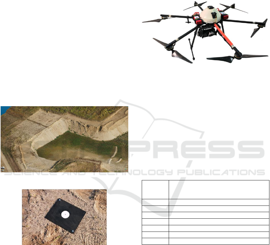
2 DATA ACQUISITION
The test-site is a part of a large sandpit located in the
Province of Pavia, in northern Italy. The selected area
roughly has a horseshoe configuration and is consti-
tuted by two flat regions connected by the excavation
front, being 10 meters high and having a slope be-
tween 30° and 90°. The upper flat zone and the scarp
are mainly bare, while the lower one shows a large
vegetated area (Figure 1). The surveyed surface is ap-
proximal 2 hectares.
Figure 1: Overview of the test site.
Figure 2: The markers.
Before the flights, 18 markers (Figure 2) were po-
sitioned and surveyed by an integrated use of classical
topography and GNSS, in a redundant way. The
GCPs' proper names range from CV1 to CV18. Their
coordinates were obtained by least-squares adjust-
ment and their precision is around 0.5 cm for the pla-
nimetric components and 1 cm for altimetry. Several
photogrammetric blocks were acquired by a UAV
equipped with a Sony A6000 camera (Figure 3), un-
der different configurations. The vehicle was made by
an Italian craftsman and has the following main char-
acteristics: 6 engines, Arducopter-compliant flight
controller, maximum payload of 1.5 kg (partly used
by the gimbal, weighting 0.3 kg), autonomy of ap-
proximately 15 minutes.
Figure 3: The HEXA-PRO UAV system operated by the
Laboratory of Geomatics at the University of Pavia.
The camera has 24 MP, a focal length of 16 mm
and a 17.5 mm GSD at the 70 m flying height. The
blocks carried out over the area are all listed in Table
1; the present paper only concerns a dataset coming
from the union of blocks 1 and 2, constituted by seven
strips. Flying height was about 70 m on average; end
lap (longitudinal) and side lap (lateral) were 77% and
60% respectively; more details can be found in (Ca-
sella and Franzini, 2016).
The Pavia group carried out the installation of the
markers, their measurement and the UAV missions.
Table 1: List of the various blocks acquired.
Block 1
North-South linear strips, at 70 metres fly-
ing height (with respect to the upper part
of the site), vertical images
Block 2
East-West linear strips, 70 m, vertical
Block 3
Radial linear strips, 70 m, vertical
Block 4
Radial linear strips, 70 m, 30° inclined
Block 5
Circular trajectory, 30 m, 45° inclined
Block 6
North-South linear strips, 40 m, vertical
Block 7
East-West linear strips, 40 m, vertical
Block 8
Radial linear strips, 40 m, vertical
3 DATA PROCESSING
The University of Pavia and the Polytechnic of Turin
decided to process the same dataset with different
software they are expert on. The Pavia unit used
Agisoft Photoscan and Trimble UAS Master, while in
Turin Pix4D, Context Capture by Bentley and Mic-
Mac were used. GCPs/CPs configuration was dis-
cussed in advance and kept fixed by both groups.
Three scenarios were considered, shown by (Figure
5, 6 and 7), according to the criteria listed below;
GISTAM 2019 - 5th International Conference on Geographical Information Systems Theory, Applications and Management
78
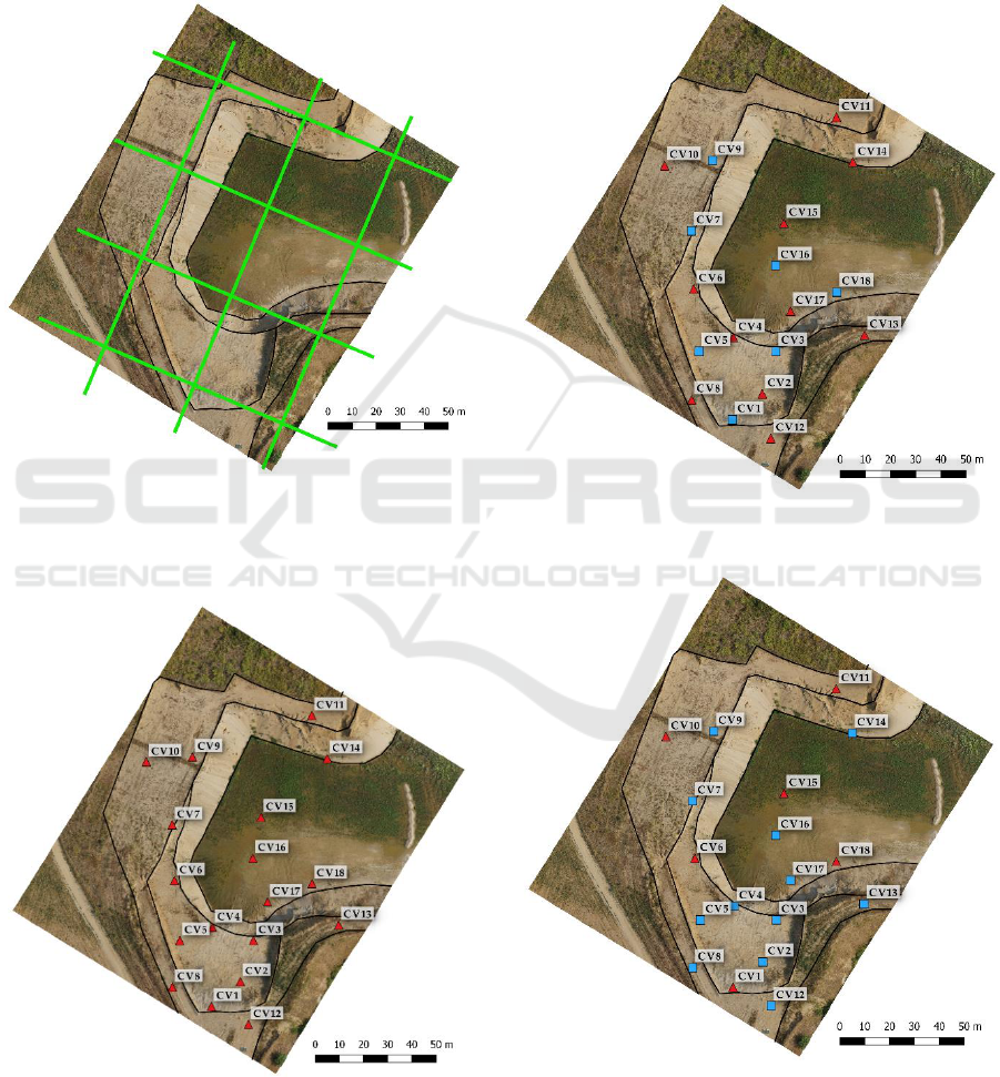
GCPs are shown in red and CPs in blue:
Configuration 1 - all the markers are used as
GCPs, to perform robust camera calibration (18
GCPs / 0 CPs);
Configuration 2 - an intermediate setup with
strong ground control and still some check points
(11 GCPs / 7 CPs);
Configuration 3 - only 6 points are used as GCPs,
that is realistic for routine surveying (6 GCPs /
12 CPs).
Other parameters and configurations were managed
independently by the two groups, namely: image
alignment, camera calibration and the adjustment
weighing. More details can be found in the next sec-
tions.
Figure 4: The block structure with three North-South and
four East-West linear strips. The images also show black
lines accounting for the main morphological features of the
sandpit.
Figure 5: Configuration 1: all the GCPs used for BBA (red
triangles).
Figure 6: Configuration 2: 11 GCPs for BBA (red triangles)
and 7 CPs for quality assessment (blue squares).
Figure 7: Configuration 3: 6 GCPs for BBA (red triangles)
and 12 CPs for quality assessment (blue squares).
Accuracy Assessment of a Photogrammetric UAV Block by using Different Software and Adopting Diverse Processing Strategies
79

3.1 The Unit of the University of Pavia
Data processing was performed with two software:
Agisoft Photoscan (rel. 1.2.4) and Inpho UAS Master
(rel. 7.0.1). The Photoscan processing will be ad-
dressed first.
When executing the photo alignment, the “High
accuracy” setup was chosen, in which tie points
were extracted from the full resolution images,
while the “Pair preselection” parameter was set
on “Generic” since no a-priori information about
imagery positions was available.
Image-point measurement was carried out in a
conservative way, meaning that, for each image,
only clearly visible points were measured. The
average number of measurements per marker
was 15 with a minimum of 9 for CV7 and a max-
imum of 29 for CV17.
Concerning camera self-calibration, after some
testing, it was decided to re-estimate camera in-
terior orientation and to adopt the parameter set
proposed as a default by the program. It is con-
stituted by the focal length (f), the corrections for
the principal point position (cx and cy), the first
three coefficients of radial distortion (K1, K2 and
K3) and the first two of tangential distortion (P1
and P2). We didn’t insert any approximate values
for the camera model, as that didn’t apparently
give any benefit.
Concerning the BBA (Bundle Block Adjust-
ment) weighting strategy, accuracy of ground-
coordinates of markers was set at 0.5 cm for the
planimetric components and 1 cm for altimetry.
For image-coordinates of manually-measured
markers, accuracy was set at ¼ of the pixel size.
Finally, for automatically-measured image-coor-
dinates of tie points, accuracy was set at 1.5 pix-
els, corresponding to three-times the overall re-
projection error. In doing so, we followed the
suggestions of the program developers, to be
adopted in the case of blurred images; we also
verified that the implemented strategy gave the
best results in terms of residuals for the CPs.
When UAS Master was used, the same setup was
used, with some exceptions. First, the program needs
to know approximate external orientation parameters:
we supplied the values calculated by PhotoScan. Tie
point extraction was performed with the “Full resolu-
tion” mode. Image-coordinates of markers were
measured by a different operator, with the same style
of being conservative and measuring only well visible
targets: the mean number of observations was 15 with
a minimum of 9 measurements on CV8 and a maxi-
mum of 26 on CV17. The parameters for camera self-
calibration are the same as those adopted for Pho-
toScan. Object-coordinates of markers were weighted
as illustrated above, but we were not able to find any
interface allowing us to fix the uncertainty of image-
coordinates of markers and tie points: we infer that
the program applies default values. We must declare
that, while we are good experts of Photoscan, we
could only use UAS Master for a few months, due to
an evaluation license. Even though maximum care
was taken, some features of the program could have
been overlooked.
3.2 The Unit of the Polytechnic of
Turin
The processing was realized using three well known
software in the scientific community: the commercial
programs Pix4D (2.1.61), Context Capture
(4.3.0.507) and the open-source tool MicMac.
The first processing was carried out using Pix4D,
where, to follow the most similar approach of the
processing steps achieved by the Pavia unit, the
following set-up was used:
For the key point extraction in the initial
processing the “Full” option was employed, this
settings means that the images were used at the
full scale, the matching image pairs according to
the input data was set-up for aerial grid and
finally, in the calibration options, the parameters
were used in the automatic/standard
configuration (automatic way to select which
key-points are extracted, standard calibration
method with an optimization of all the internal
parameters (since is well known that the camera
used with UAVs, are much more sensitive to
temperature or vibrations, which affect the
camera calibration, as a consequence it is
recommended to select this option when
processing images taken with such cameras)).
Finally, the rematch option that allows to add
more matches after the first part of the initial
processing, which usually improves the quality
of the reconstruction was used as well (this part
is important not in the first alignment but for
improving it after the GCPs measurements);
Image-point measurement was carried out
according to the strategy followed by Pavia unit,
in this case the average number of measurements
per marker was 26 with a minimum of 15 for
CV10 and a maximum of 40 for CV17.
The next step was the BBA (bundle block
adjustment), for this step-in order to fix a
weighting for the two components, according to
the accuracy of the measured coordinates of the
GISTAM 2019 - 5th International Conference on Geographical Information Systems Theory, Applications and Management
80

markers the horizontal accuracy was set at 0.5 cm
while the vertical accuracy was fixed at 1 cm. It
is not possible in Pix4D to set the accuracy of the
measurement on the images, probably this value
as commonly used is fixed at ½ of the pixel size.
During the BBA the camera self-calibration is
calculated as well, in this case the parameter set
as default has been used. The final results of the
camera calibration in Pix4D could be extracted
from the final report and are related to the focal
length (f), the corrections for the principal point
position (cx and cy), the first three coefficients of
radial distortion (K1, K2 and K3 called R1 R2
and R3 in Pix4d) and the first two of tangential
distortion (P1 and P2 called T1 and T2 in Pix4d).
The second commercial employed software was
Context Capture by Bentley System, the approach
followed by this program is similar to the one
described above and is summarized in the following
points:
The first alignment has been performed using the
default setting with “High” density in the key
point extraction (scale image size), in this first
step the software starting from the information
derived by the EXIF file adjust the camera
internal parameters as well (f, cx, cy, K1, K2, K3,
P1 and P2).
After the first processing step the camera pose
were estimated in an arbitrary coordinate system,
the next step was the image-point measurements.
In order to help the operator in the measurement
phase this part was performed first of all using
three GCPs in three different images and then a
rigid registration was performed. Starting from
this first results an accurate measurement of the
other points has been achieved, the average
number of measurements per marker was 15 with
a minimum of 9 for CV10 and a maximum of 33
for CV17.
The BBA weighting for the two components, was
in the horizontal component 0.5 cm while the
vertical one was fixed at 1 cm (the same settings
of the other employed commercial software).
During the BBA the camera optimization has
been performed as well to define the internal
parameters of the employed camera.
Furthermore, according to the actual trend in the
Geospatial information area that even more move the
attention to the open-source software and tools in the
presented test the open source software MicMac has
been employed. The software has been developed by
the MATIS laboratory (IGN France) and it has been
delivered as open source in 2007, usable in different
contexts (satellite, aerial, terrestrial) for extracting
point clouds from images (Pierrot-Deseilligny and
Clery, 2011). The pipeline of the software (Rupnik et
al., 2017) is quite different comparing to the
commercial one since all the commands in the
employed version (5348 for Ubuntu) need to be
inserted by the terminal. In the following points, a
short list of the used simplified tools is reported :
The first used tool was Tapioca, with this
command MicMac computing the tie points on
the images. The options that could be used in
Tapioca are the strategy for extracting the
information from the images (All, MulScale
etc..) and the number of pixel that we need to use
for extracting the tie points. In the present test all
the possible pairs were analysed (options All)
and in order to speed up the process the images
were resampled at 1500 pixel (another option
decided during the process).
After Tapioca only the tie points are extracted, to
align the images according to the extracted points
another tool need to be launch: Tapas. This
command allows to calibrate the images and to
align it in a local reference system according to
several parameters. A simple use of Tapas has
been carried out using as calibration model the
Fraser approach (Fraser, 1997). This is a radial
model, with decentric and affine parameters the
model has 12 degrees of freedom: 1 for focal
length, 2 for principal point, 2 for distortion
centre, 3 for coefficients of radial distortion (r3,
r5, r7), 2 for decentric parameters, 2 for affine
parameters, in this calibration model the PPA
(Principal Point of Autocollimation) and PPS
(Principal Point of Simmetry) are considered not
equal. The next step was the image-point
measurements. This part was performed in two
steps using an approach similar to the one used
in Context Capture: first of all, using three GCPs
in three different images a rigid registration was
performed (using SaisieAppuisInit for image
measurements and GCPBascule for the rigid
registration). Starting from this first results an
accurate measurement of the other points has
been achieved (SaisieAppuisPredict), the
average number of measurements per marker
was 18 with a minimum of 12 for CV10 and a
maximum of 30 for CV17.
Finally, for performing the BBA the weighting
factor for the two components was fixed at 1 cm
(is not possible in MicMac adopt different weight
for the horizontal and vertical components). For
image-coordinates of manually-measured
markers the accuracy was set at ½ of the pixel
size. During the BBA in MicMac as interior
Accuracy Assessment of a Photogrammetric UAV Block by using Different Software and Adopting Diverse Processing Strategies
81

calibration parameters the ones derived from the
first orientation process were used.
4 BUNDLE BLOCK
ADJUSTMENT RESULTS
The quality of aerial triangulation was mainly
evaluated by assessing the differences between the
photogrammetrically-measured and the ground-
surveyed object-coordinates of GCPs and CPs.
Outlier rejection was preliminary performed, based
on robust statistics, by means of an in-house Matlab
tool developed at the University of Pavia. For each
component, X, Y and Z, the average value 𝑚 of the
residual was determined by means of the median
operator. The standard deviation 𝜎 was also
estimated, by multiplying the MAD (Mean Absolute
Deviation) of the residuals by the factor 1.4826
(Hampel, 1974). The confidence interval was
determined, having the form [𝑚 − 𝑛 ∙ 𝜎, 𝑚 + 𝑛 ∙ 𝜎],
where the 𝑛 coefficient was set at 2.5758,
corresponding to the 99% probability under the
normality condition. It must be said that all the
measurements considered resulted to be inliers.
Table 2: Main statistical figures for GCP/CP residuals for Configuration 1.
Config 1: GCP 18
GCP
CP
X [m]
Y [m]
Z [m]
X [m]
Y [m]
Z [m]
Photoscan
mean
0.000
0.000
0.000
-
-
-
std
0.003
0.003
0.009
-
-
-
rmse
0.003
0.003
0.009
-
-
-
UAS Master
mean
0.000
0.000
0.000
-
-
-
std
0.003
0.002
0.008
-
-
-
rmse
0.003
0.002
0.008
-
-
-
Pix4D
mean
0.000
0.000
-0.001
-
-
-
std
0.004
0.005
0.010
-
-
-
rmse
0.004
0.005
0.010
-
-
-
Context Capture
mean
0.000
0.000
0.000
-
-
-
std
0.004
0.004
0.009
-
-
-
rmse
0.004
0.004
0.009
-
-
-
MicMac
mean
0.000
0.000
0.000
-
-
-
std
0.002
0.002
0.002
-
-
-
rmse
0.002
0.002
0.002
-
-
-
Table 3: Main statistical figures for GCP/CP residuals for Configuration 2.
Config 2: GCP 11/CP 7
GCP
CP
X [m]
Y [m]
Z [m]
X [m]
Y [m]
Z [m]
Photoscan
mean
0.000
0.000
0.000
-0.001
-0.001
-0.001
std
0.003
0.003
0.009
0.004
0.005
0.013
rmse
0.003
0.003
0.009
0.004
0.005
0.013
UAS Master
mean
0.000
0.000
0.000
0.002
-0.001
0.010
std
0.003
0.003
0.008
0.007
0.004
0.017
rmse
0.003
0.003
0.008
0.007
0.004
0.020
Pix4D
mean
0.000
0.000
-0.001
0.002
0.002
0.003
std
0.004
0.005
0.008
0.005
0.007
0.015
rmse
0.004
0.005
0.008
0.005
0.007
0.015
Context Capture
mean
0.001
-0.001
0.000
0.001
-0.002
-0.003
std
0.005
0.004
0.009
0.009
0.007
0.012
rmse
0.005
0.004
0.009
0.009
0.007
0.012
MicMac
mean
0.000
0.000
0.002
-0.004
0.005
0.047
std
0.005
0.006
0.010
0.007
0.011
0.083
rmse
0.005
0.006
0.011
0.008
0.012
0.096
GISTAM 2019 - 5th International Conference on Geographical Information Systems Theory, Applications and Management
82
Table 4: Main statistical figures for GCP/CP residuals for Configuration 3.
Config 3: GCP 6/CP 12
GCP
CP
X [m]
Y [m]
Z [m]
X [m]
Y [m]
Z [m]
Photoscan
mean
0.000
0.000
0.000
-0.001
-0.005
-0.007
std
0.001
0.004
0.006
0.004
0.004
0.016
rmse
0.001
0.004
0.006
0.004
0.006
0.017
UAS Master
mean
0.000
-0.001
0.002
0.001
0.00
0.007
std
0.007
0.005
0.015
0.005
0.004
0.023
rmse
0.007
0.005
0.015
0.005
0.004
0.024
Pix4D
mean
0.000
0.001
-0.001
-0.001
0.001
0.002
std
0.004
0.008
0.008
0.005
0.005
0.014
rmse
0.004
0.008
0.008
0.005
0.005
0.014
Context Capture
mean
-0.003
0.002
0.011
-0.007
0.000
0.020
std
0.007
0.005
0.027
0.009
0.007
0.037
rmse
0.008
0.005
0.029
0.011
0.007
0.042
MicMac
mean
0.000
-0.001
0.002
0.000
0.003
0.056
std
0.003
0.005
0.012
0.015
0.017
0.090
rmse
0.003
0.005
0.012
0.015
0.017
0.106
Table 5: Main statistical figures for GCP/CP residuals for Photoscan.
Photoscan
GCP
CP
X [m]
Y [m]
Z [m]
X [m]
Y [m]
Z [m]
Config 1
[GCP:18/18]
mean
0.000
0.000
0.000
-
-
-
std
0.003
0.003
0.009
-
-
-
rmse
0.003
0.003
0.009
-
-
-
Config 2
[GCP:11/11;
CP:7/7]
mean
0.000
0.000
0.000
-0.001
-0.001
-0.001
std
0.003
0.003
0.009
0.004
0.005
0.013
rmse
0.003
0.003
0.009
0.004
0.005
0.013
Config 3
[GCP:6/6;
CP:12/12]
mean
0.000
0.000
0.000
-0.001
-0.005
-0.007
std
0.001
0.004
0.006
0.004
0.004
0.016
rmse
0.001
0.004
0.006
0.004
0.006
0.017
Table 6: Main statistical figures for GCP/CP residuals for UAS Master.
UAS Master
GCP
CP
X [m]
Y [m]
Z [m]
X [m]
Y [m]
Z [m]
Config 1
[GCP:18/18]
mean
0.000
0.000
0.000
-
-
-
std
0.003
0.002
0.008
-
-
-
rmse
0.003
0.002
0.008
-
-
-
Config 2
[GCP:11/11;
CP:7/7]
mean
0.000
0.000
0.000
0.002
-0.001
0.010
std
0.003
0.003
0.008
0.007
0.004
0.017
rmse
0.003
0.003
0.008
0.007
0.004
0.020
Config 3
[GCP:6/6;
CP:12/12]
mean
0.000
-0.001
0.002
0.001
0.00
0.007
std
0.007
0.005
0.015
0.005
0.004
0.023
rmse
0.007
0.005
0.015
0.005
0.004
0.024
Table 7: Main statistical figures for GCP/CP residuals for Pix4D.
Pix4D
GCP
CP
X [m]
Y [m]
Z [m]
X [m]
Y [m]
Z [m]
Config 1
[GCP:18/18]
mean
0.000
0.000
-0.001
-
-
-
std
0.004
0.005
0.010
-
-
-
rmse
0.004
0.005
0.010
-
-
-
Config 2
[GCP:11/11;
CP:7/7]
mean
0.000
0.000
-0.001
0.002
0.002
0.003
std
0.004
0.005
0.008
0.005
0.007
0.015
rmse
0.004
0.005
0.008
0.005
0.007
0.015
Config 3
[GCP:6/6;
CP:12/12]
mean
0.000
0.001
-0.001
-0.001
0.001
0.002
std
0.004
0.008
0.008
0.005
0.005
0.014
rmse
0.004
0.008
0.008
0.005
0.005
0.014
Accuracy Assessment of a Photogrammetric UAV Block by using Different Software and Adopting Diverse Processing Strategies
83
Table 8: Main statistical figures for GCP/CP residuals for Context Capture.
zContext Capture
GCP
CP
X [m]
Y [m]
Z [m]
X [m]
Y [m]
Z [m]
Config 1
[GCP:18/18]
mean
0.000
0.000
0.000
-
-
-
std
0.004
0.004
0.009
-
-
-
rmse
0.004
0.004
0.009
-
-
-
Config 2
[GCP:11/11;
CP:7/7]
mean
0.001
-0.001
0.000
0.001
-0.002
-0.003
std
0.005
0.004
0.009
0.009
0.007
0.012
rmse
0.005
0.004
0.009
0.009
0.007
0.012
Config 3
[GCP:6/6;
CP:12/12]
mean
-0.003
0.002
0.011
-0.007
0.000
0.020
std
0.007
0.005
0.027
0.009
0.007
0.037
rmse
0.008
0.005
0.029
0.011
0.007
0.042
Table 9: Main statistical figures for GCP/CP residuals for MicMac.
MicMac
GCP
CP
X [m]
Y [m]
Z [m]
X [m]
Y [m]
Z [m]
Config 1
[GCP:18/18]
mean
0.000
0.000
0.000
-
-
-
std
0.002
0.002
0.002
-
-
-
rmse
0.002
0.002
0.002
-
-
-
Config 2
[GCP:11/11;
CP:7/7]
mean
0.000
0.000
0.002
-0.004
0.005
0.047
std
0.005
0.006
0.010
0.007
0.011
0.083
rmse
0.005
0.006
0.011
0.008
0.012
0.096
Config 3
[GCP:6/6;
CP:12/12]
mean
0.000
-0.001
0.002
0.000
0.003
0.056
std
0.003
0.005
0.012
0.015
0.017
0.090
rmse
0.003
0.005
0.012
0.015
0.017
0.106
Results are shown here, grouped in two different
ways, to favourite analysis and comparisons. Tables
2-4 group results per configuration. Table 2 shows,
for instance, results concerning GCPs and CPs for all
the programs considered and only for Configuration
1. We show the name of the program used, the mean,
standard deviation and RMSE of the difference
between the photogrammetrically-obtained object-
coordinates of markers and those determined by
surveying; the analysis is performed for all the X, Y
and Z components of GCPs and CPs, if any
Tables 5-9 illustrate the behaviour of the same
program through the configurations depicted. Table 5
shows, for instance, results concerning Photoscan for
all the three scenarios. We report the name of the
configuration with the number of the GCPs and CPs
used, the mean, standard deviation and RMSE values
as explained above.
Figure 8 graphically summarizes results for the
three configurations and five programs, in terms of
RMSE. For readability reason, the axis of ordinates
of the second and third graph is limited to 4.5 cm,
while altimetric results for MicMac are larger, around
10 cm.
The figures shown suggest several remarks, some
straightforward and others surprising.
Horizontal components always perform better
than Z. The only exception is constituted by Mic-
Mac in Configuration 1, where all coordinates
show the same accuracy.
It is well known that BBA estimates the orienta-
tion parameters in order to reach the best fitting
between the photogrammetric and topographic
coordinates of GCPs. A widely accepted rule
states that accuracy figures for GCPs underesti-
mate the actual ones. Therefore, it is useful and
recommended to use independent check points in
order to perform a reliable accuracy assessment.
Our results confirm the mentioned general rule,
but discrepancies between GCPs and CPs (for
Configuration 2 and 3, only) are less evident than
expected, especially for the planimetric compo-
nents. This probably means that the statistics on
GCPs can be considered a good quality estima-
tor, at least for X and Y coordinates.
The decreasing number of GCPs influences re-
sults, as expected. The different programs con-
sidered behave in a different way, according to
this aspect. Photoscan, UAS Master and Pix4D
always show good results while Context Capture
has significant quality degradation in the altimet-
ric component when passing from 11 to 6 GCPs
(Table 8). Furthermore, the program shows
anomalous values for Z in Configuration 3. Mic-
GISTAM 2019 - 5th International Conference on Geographical Information Systems Theory, Applications and Management
84
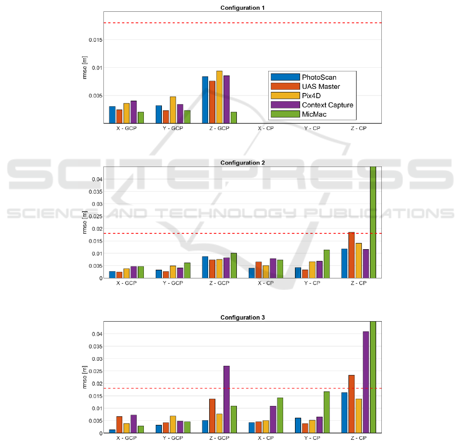
Mac presents good results for X and Y compo-
nents but large residuals for Z, probably this
aspect is connected to the calibration model used
in MicMac. A strategy more similar to the one
performed by the other used programs, like the
FraserBasic model with PPA=PPS, should be
reconsider as a best option where a little number
of GCPs are used for the BBA.
The GSD for the considered imagery is around
1.8 cm and is represented with a red dashed line
in the figures. RMSE values are almost always
below the GSD value, thus highlighting that re-
sults are good in general. In Configuration 1,
RMSE figures are all below the GSD threshold,
for all the components and the programs adopted.
Configuration 2 shows similar results also for al-
timetric component with an exception for Mic-
Mac software. In Configuration 3, all RMSE fig-
ures are within the GSD threshold apart from the
Z component for ContextCapture (for both GCPs
and CPs) and the Z of CPs for MicMac.
Figure 8: A summary of the obtained results. Histograms show the RMSE for the three-considered configurations; bars are
coloured according to the software and the red dashed line represents the GSD value. The y-axis of Configuration 2 and 3 is
limited to 4.5 cm for readability reason while the altimetric results on CPs for MicMac are larger.
Accuracy Assessment of a Photogrammetric UAV Block by using Different Software and Adopting Diverse Processing Strategies
85

5 CONCLUSIONS AND FURTHER
ACTIVITIES
A significant part of a sandpit was surveyed by a
UAV equipped with a Sony A6000 camera. A set of
ground points were measured and used either for
block orientation or quality assessment.
Five software were compared: Photoscan, UAS
Master, Pix4D, Context Capture and MicMac. They
were used to perform BBA in three configurations
characterized by a different ratio between GCPs and
CPs. In Configuration 1, markers were all used as
GCPs to perform robust camera calibration; Configu-
ration 2 deals with an intermediate setup with strong
ground control and some check points; Configuration
3 is the more realistic one and simulates a routine sur-
veying.
For each program, BBA strategy was carefully
studied and final settings, described in Section 3,
were tuned to optimize results. Residuals between the
photogrammetrically-obtained object-coordinates of
markers and those determined by surveying were
formed and analysed.
Results for Photoscan, Pix4D and UAS Master
are good, less than 1 GSD for the planimetric compo-
nents and less than 1.5 GSD, at worst, for the altimet-
ric one. Context Capture shows similar results for X
and Y while the Z coordinate presents larger residuals
especially for Configuration 3. Finally, MicMac
shows anomalous residuals in the altimetric compo-
nent for both Configuration 2 and 3; such values will
be further investigated, using different calibration
strategies to better evaluate the results in more similar
conditions.
The decreasing number of GCPs influences re-
sults, as expected. Photoscan, UAS Master and Pix4D
always show good results while Context Capture and
MicMac present good results for X and Y compo-
nents but large residuals for Z.
Further activities will follow two directions. On
one hand, the other flights described in Table 1 will
be processed with attention on oblique blocks to in-
vestigate their influence on final accuracy. On the
other, final products, such as dense point clouds, will
be assessed to explore the influence of BBA parame-
ters in their generation. Several check points (more
than 250) were already measured with a topographic
total station on the upper flat area and on the scarp of
the sandpit. An accurate comparison between the
achieved point clouds and these points will be per-
formed. Finally, an evaluation of point density will be
realized comparing the clouds obtained in flat or
scarp areas.
ACKNOWLEDGEMENT
The VAGA Srl company, being the owner of the sur-
veyed sandpit, is here acknowledged for hosting the
test. We are pleased to mention Eng. Emanuele Della
Pasqua, Dr. Enrico Parmini, Dr. Maurizio Visconti,
Surveyor Andrea Montemartini.
We are also pleased to thank two technicians of
the Laboratory of Geomatics, Paolo Marchese and
Giuseppe Girone for strongly supporting some phases
of the described test: the manufacturing, placing and
surveying of the markers, UAV management and data
acquisition.
The authors' contribution was equal in the defini-
tion and drafting of the article. The processing was
conducted in a coordinated but independent way by
the two universities involved, as illustrated in Section
3.
REFERENCES
Benassi, F., Dall’Asta, E., Diotri, F., Forlani, G., Morra di
Cella, U., Roncella, R., Santise, M., 2017. Testing
accuracy and repeatability of UAV blocks oriented with
GNSS-supported aerial triangulation. In Remote
Sensing, 9(2), 172.
Casella, V., Franzini, M., 2016. Modelling steep surfaces
by various configurations of nadir and oblique
photogrammetry. In ISPRS Annals of Photogrammetry,
Remote Sensing and Spatial Information Sciences, 3(1).
Fraser, C., 1997. Digital camera self-calibration. In ISPRS
Journal of Photogrammetry and Remote Sensing, vol.
52, issue 4, pp. 149-159
Gini, R., Pagliari, D., Passoni, D., Pinto, L., Sona, G.,
Dosso, P., 2013. UAV photogrammetry: Block
triangulation comparisons. In Int. Arch. Photogram.
Remote Sens. Spat. Inf. Sci, 1, W2.
Hampel, F.R., 1974. The influence curve and its role in
robust estimation. In Journal of the American statistical
association, 69(346), 383-393.
James, M. R., Robson, S., d'Oleire-Oltmanns, S.,
Niethammer, U., 2017. Optimising UAV topographic
surveys processed with structure-from-motion: Ground
control quality, quantity and bundle adjustment. In
Geomorphology, 280, 51-66.
Lucieer, A., Jong, S.M.D., Turner, D., 2014. Mapping
landslide displacements using Structure from Motion
(SfM) and image correlation of multi-temporal UAV
photography. In Progress in Physical Geography,
38(1), 97-116.
Nex, F., Remondino, F., 2014. UAV for 3D mapping
applications: a review. In Applied geomatics, 6(1), 1-
15.
Nocerino, E., Menna, F., Remondino, F., Saleri, R., 2013.
Accuracy and block deformation analysis in automatic
UAV and terrestrial photogrammetry-Lesson learnt. In
GISTAM 2019 - 5th International Conference on Geographical Information Systems Theory, Applications and Management
86

ISPRS Annals of the Photogrammetry, Remote Sensing
and Spatial Information Sciences, 2(5/W1), 203-208.
Pierrot-Deseilligny, M., Clery, I., 2011. APERO, an Open
Source Bundle Adjusment Software for Automatic
Calibration and Orientation of a Set of Images. In
ISPRS Archives, International Workshop 3D-ARCH,
on CD-ROM, Trento, Italy
Rangel, J. M. G., Gonçalves, G. R., Pérez, J. A., 2018. The
impact of number and spatial distribution of GCPs on
the positional accuracy of geospatial products derived
from low-cost UASs. In International journal of remote
sensing, 39(21), 7154-7171.
Remondino, F., Barazzetti, L., Nex, F., Scaioni, M.,
Sarazzi, D., 2011. UAV photogrammetry for mapping
and 3d modeling–current status and future perspectives.
In International Archives of the Photogrammetry,
Remote Sensing and Spatial Information Sciences,
38(1), C22.
Rupnik, E., Daakir, M., Deseilligny, M. P., 2017. MicMac–
a free, open-source solution for photogrammetry. In
Open Geospatial Data, Software and Standards, 2(1),
14.
Samad, A.M., Kamarulzaman, N., Hamdani, M.A., Mastor,
T. A., Hashim, K.A., 2013. The potential of Unmanned
Aerial Vehicle (UAV) for civilian and mapping
application. In System Engineering and Technology
(ICSET), 2013 IEEE 3rd International Conference on,
313-318.
Tahar, K. N., 2013. An evaluation on different number of
ground control points in unmanned aerial vehicle
photogrammetric block. In Int. Arch. Photogramm.
Remote Sens. Spat. Inf. Sci, 40, 93-98.
Verykokou, S., Ioannidis, C., Athanasiou, G., Doulamis,
N., Amditis, A., 2018. 3D reconstruction of disaster
scenes for urban search and rescue. Multimedia Tools
and Applications, 77(8), 9691-9717.
Zongjian, L.I.N., 2008. UAV for mapping-low altitude
photogrammetric survey. In International Archives of
Photogrammetry and Remote Sensing, Beijing, China,
37, 1183-1186.
Accuracy Assessment of a Photogrammetric UAV Block by using Different Software and Adopting Diverse Processing Strategies
87
