Analyzing Traffic Signal Performance Measures to Automatically
Classify Signalized Intersections
Dhruv Mahajan
1
, Tania Banerjee
1
, Anand Rangarajan
1
, Nithin Agarwal
2
, Jeremy Dilmore
3
,
Emmanuel Posadas
4
and Sanjay Ranka
1
1
Department of Computer Science & Engineering, University of Florida, Gainesville, U.S.A.
2
Transportation Institute, University of Florida, Gainesville, U.S.A.
3
Florida Department of Transportation, Deland, U.S.A.
4
City of Gainesville, Gainesville, U.S.A.
Keywords:
ATSPM, Clustering, Classification, Signal Performance, Intersection.
Abstract:
Traffic signals are installed at road intersections to control the flow of traffic. An optimally operating traffic
signal improves the efficiency of traffic flow while maintaining safety. The effectiveness of traffic signals has
a significant impact on travel time for vehicular traffic. There are several measures of effectiveness (MOE)
for traffic signals. In this paper, we develop a work-flow to automatically score and rank the intersections in a
region based on their performance, and group the intersections that show similar behavior, thereby highlighting
patterns of similarity. In the process, we also detect potential bottlenecks in the region of interest.
1 INTRODUCTION
Traffic signals are ubiquitous in managing vehicular
and pedestrian traffic at an intersection where two or
more road segments meet. The signals are controlled
by sophisticated controller devices that are mounted
inside a cabinet that is co-located at every intersec-
tion. Traffic signal controllers eliminate conflicts
(protected phase) or reduce conflicts between move-
ments by displaying signal indications to assign ap-
propriate right of way. These displays can be based on
fixed signal timing parameters to maintain consistent
intervals or it can be based on actuated signal timing
parameters to account for varying demand. In addi-
tion, some traffic signal controllers have the capabil-
ity to log every signal phase change and every vehicle
detector actuation at a high resolution.
Automated Traffic Signal Performance Measures
(ATSPM) (UDOT, 2017) is a tool being deployed in
a slew of traffic controllers that enhances traffic sig-
nal management by using the high-resolution (10Hz)
controller logs to generate operational performance
measures. The system—due to its capability of mon-
itoring traffic events at a high resolution—opens a
broader range of possibilities that were not available
in previous systems which dealt with aggregated data
at a coarser level of granularity. In this paper we show
how the high resolution data may be used in ways
that can vastly reduce manual intervention typically
needed for traffic and intersection monitoring.
There are several measures of effectiveness
(MOE) for traffic signals that are studied in the lit-
erature and used in the field; these MOE’s rely on
ATSPM or otherwise to assess the efficacy of the sig-
nal timing parameters of a controller. The measures
are computed using data collected at the intersection
(by signal controllers and vehicle detectors) and help
highlight specific characteristics such as green phase
utilization. In our paper, we use split failures as the
primary MOE to develop our work-flow and then ac-
centuate the data further using measures such as ar-
rivals on red and arrivals on green. Split failures oc-
cur when there is a vehicle queue at the intersection
at the end of the maximum allotted green time for one
direction.
The contributions in this paper are summarized as
follows.
1. We develop a novel work-flow based on data ana-
lytics techniques that allow us to process raw AT-
SPM data from a region and automatically quan-
tify and visualize the performance of the signals
that they represent. This is achieved by using de-
138
Mahajan, D., Banerjee, T., Rangarajan, A., Agarwal, N., Dilmore, J., Posadas, E. and Ranka, S.
Analyzing Traffic Signal Performance Measures to Automatically Classify Signalized Intersections.
DOI: 10.5220/0007714701380147
In Proceedings of the 5th International Conference on Vehicle Technology and Intelligent Transport Systems (VEHITS 2019), pages 138-147
ISBN: 978-989-758-374-2
Copyright
c
 2019 by SCITEPRESS – Science and Technology Publications, Lda. All rights reserved

mand based split failures as an MOE and develop
algorithms to characterize the performance of an
intersection on this basis.
2. We deploy clustering techniques to group signals
with the same performance or behavior together.
Clustering is carried out along both space and
time. Thus, the work-flow, while automatically
finding spatial and temporal patterns in the data,
also highlights signals that need attention in terms
of coordination adjustment or fixing of detection
errors.
3. We use a classifier to further classify the signals
based on whether they cater to high or low traf-
fic demand (based on split failures) and exhibit
high or low utilization of green time (based on the
ratio arrivals on red/arrivals on green). This al-
lows us to categorize the intersections into one of
four categories, briefly described below: (i) sig-
nals that perform well, (ii) signals that serve high
demand with no simple remedy, (iii) signals that
serve high demand but show a potential coordina-
tion issue, and lastly (iv) signalized intersections
with low demand but a potential coordination is-
sue.
This work provides an analytics and visualization
model that creates a bird’s eye view of the perfor-
mance of arterial street networks for traffic engineers.
This is useful since the problematic intersections can
be easily spotted. At this point, the performance
charts generated automatically by the current ATSPM
system can be analyzed to further study the problem.
Thus, our work enables a traffic engineer or manager
to be more proactive with respect to the problems ex-
perienced in the network. It eliminates the need to
rely on complaint calls and the need to sift through
all the ATSPM generated charts and measures for all
the intersections on a regular basis to actively identify
issues.
The rest of the paper is organized as follows. Sec-
tion 2 presents the related work in traffic engineering.
Section 3 details the algorithmic framework for the
study, while Section 4 presents the case studies with
conclusions presented in Section 5.
2 RELATED WORK
Evaluating the performance of traffic signal systems
is important for identifying any problems and ad-
dressing them, as well as for assessing and planning
enhancements to these systems. Radivojevic et al.
in (Radivojevic and Stevanovic, 2017), presents an
evaluation framework for a comprehensive quantita-
tive evaluation that may be used to examine the per-
formance of the agencies’ that are responsible for the
functioning of these signals. Our work in this pa-
per is different as it presents an automatic evalua-
tion, analysis and notification system for signal per-
formance using high resolution data from signal con-
trollers and detectors. This will allow traffic engineers
to be proactive in addressing issues, instead of ad-
dressing these passively as a result of user feedback.
2.1 Arterial and Network Evaluation
Purdue Coordination Diagrams (PCDs), Arrivals on
Green vs Red and other such measures (US Depart-
ment of Transportation, 2013; Day et al., 2014) give
us a precise idea of the arrivals of vehicles and the cor-
responding signal phase. However a practitioner has
to generate and analyze the diagram for each direc-
tion of movement at every intersection to analyze sig-
nal performance. Our method presented in this paper
would automatically detect the problem areas, which
allows the practitioner to review only the diagrams for
specific intersections and movements. Howell Li et
al. (Li et al., 2017) present a heuristic based on system
wide split failure identification and evaluation. By us-
ing this heuristic, they demonstrated performance im-
provements for specific corridors. This paper builds
upon this approach and enhances it by proposing an
automated way to categorize all intersections in a net-
work based on split failures and hence preemptively
identify any corridors that may be under-performing.
2.2 Measures of Effectiveness (MOE)
Several MOE are used in the field and a detailed de-
scription of these are available at (US Department of
Transportation, 2013; Day et al., 2014). In this paper,
we focus on the split status (specifically, split failure)
because it is a good yardstick of how well an inter-
section services the vehicles. It is also very simple to
monitor, and this data is generally available for most
of the intersections. In addition, our methodology is
general enough and may be easily extended to another
MOE or a combination of MOE’s.
2.3 ATSPM and other Data Analytics
Efforts
Data analytics techniques have been previously ap-
plied to traffic flows and here we present the rele-
vant application areas. Wemegah et al. (Wemegah
and Zhu, 2017) present techniques for management
of big data for analyzing traffic volumes and conges-
tion, addressing all the steps in the analytics pipeline
Analyzing Traffic Signal Performance Measures to Automatically Classify Signalized Intersections
139

namely, data acquisition, data storage, data cleaning,
data analysis and visualization. Amini et al. (Amini
et al., 2017) describe an architecture for real time traf-
fic control. Machine learning techniques have been
applied for predicting traffic flows and thereby traf-
fic congestion. Horvitz et al. (Horvitz et al., 2005)
presents a probabilistic traffic forecasting system us-
ing Bayesian structure search. Huang et al. (Huang
et al., 2018)propose a set of new, derived MOE’s that
are designed to measure health, demand and control
problems in signalized intersections. The newly pro-
posed MOE’s are based on approach volume and pla-
tooning data derived from ATSPMs (UDOT, 2017).
Our approach, in sharp contrast, is based on existing
MOE’s for split status and targets the differences be-
tween arrivals on red vs arrivals on green. Our ap-
proach automatically highlights potential demand and
coordination problems in the network.
3 ALGORITHMIC FRAMEWORK
We describe the data analytics techniques and infras-
tructure in this section. This work-flow is used to au-
tomatically determine how well the signal is function-
ing and also flag the potentially problematic intersec-
tions.
3.1 Processing Data from Intersections
Pre-processing. We first describe the method to an-
alyze performance for an individual signalized inter-
section. We use multiple MOE’s to model and quan-
tify the performance of signals. In particular, we use
split failures (Max-outs/Force-offs), in combination
with arrivals on red and arrivals on green (AoR/AoG).
In actuated operation, a Max-out is said to have oc-
curred when a phase (directional flow) terminates be-
cause the phase reaches the maximum green time due
to continued demand. A Max-out event almost always
indicates a high demand. It can also be an indica-
tion of a situation where demand is at capacity or over
the capacity of the phase (assuming no major timing
problems). However, a set of intersections on a cor-
ridor may be coordinated to allow maximal flow of
traffic on the major street. In such cases, the phases
2 and 6(Figure 1) corresponding to major street flow
will always use the max green time. Force-offs occur
when a phase terminates after reaching the maximum
green time allocated to it yet the demand is not ful-
filled. Arrivals on red or green give us a count of how
many cars arrived at a phase of an intersection when
that phase was green versus how many arrived when
the phase was red. An intersection with fewer split
Figure 1: Phase Diagram: Vehicular & pedestrian move-
ment at four way intersections. (US Department of Trans-
portation, 2008).
failures and higher arrivals on green is, in general, a
highly utilized intersection. On the other hand, a large
number of Max-outs or Force-offs along a phase or a
high ratio of arrivals on red versus arrivals on green
indicates a congestion situation, which may or may
not be remediable. In addition to split failures and
AoR/AoG, we also record the pedestrian-begin-walk
events because these events may help explain reduced
throughput for some intersections at certain times of
the day (when coordination is lost due to pedestrian
calls).
Our analysis is based on split failures for the
phases (Figure 1) 2, 4, 6, and 8 and AoRs and AoGs
on the major phases 2 and 6. AoRs and AoGs were
considered for phases 2 and 6 because these are typ-
ically mapped to the primary street and the vehicle
detection data available included only phases 2 and 6.
Aggregation. In our methodology, we first aggre-
gate the high resolution (10Hz) data from ATSPM
into minute by minute buckets. For reported split fail-
ures in a phase (Max-outs/Force-offs), we record a
value of 1 if that phase fails during the minute under
consideration. More than one split failure in a minute
is also recorded as a 1. If there are no split failures
reported for the phase, we record a value of 0. We
ignore the split failures reported in some coordinated
corridors when there is no demand (max recall). This
is done by recording any detector − on events in the
seconds preceding the reported split failure. This is
similar to the Red Occupancy Ratio (RoR) which is
widely used in the literature and in practice (Smaglik
et al., 2011) In the rest of the paper, the word split fail-
ure refers only to these demand based split failures.
The number of vehicles that arrived at the minute be-
ing considered on a red signal is reported as AoR.
Similarly, the number of vehicles that arrived at that
minute on green is recorded as AoG. For pedestrian
events, we score the pedestrian begin walk event with
VEHITS 2019 - 5th International Conference on Vehicle Technology and Intelligent Transport Systems
140

a value of 1 if the event occurred in the minute under
consideration. This gives us a measure of pedestrian
demand during the minute under consideration. Here,
programmed pedestrian calls (ped recall) events were
not eliminated and it is assumed that all events are an
indication of pedestrian demand. The next step in our
methodology is to create a 1440 bit long binary fea-
ture vector for each phase, intersection for the whole
day. The dimensionality is 24 × 60 = 1440. Hence,
we will have such a vector for each day that we study
the intersection. Furthermore, to eliminate isolated
split failure events (outliers) and highlight windows
of poor performance, we process this vector through
a sliding window algorithm that extracts contiguous
chunks of 0s and 1s from the vector.
Smoothening. The sliding window algorithm is
presented as Algorithm 1. There are three inputs to
this algorithm. These are: (i) the binary feature vector
v representing split failure events for a phase during
the day, (ii) wSize, the size of the window, and (iii)
th, a threshold parameter representing the minimum
number of Split Failures in the window for all bits
in that window to be considered as 1. The algorithm
will output an ordered list of indices such that each
index gives a position in v where a contiguous sec-
tion of 1’s either begins or ends in the corresponding
smoothed vector. The first index in the output list cor-
responds to the position of the first 1 in the smoothed
output vector. Using the ordered list of indices that
is output by this algorithm, one can easily construct
the smoothed vector corresponding to a feature vec-
tor. Figure 2 presents a simple example demonstrating
the functioning of the algorithm. For an input vector
111110000110, window size 6 and threshold 5, the
algorithm outputs the list {0,5} from which the cor-
responding smoothed output vector is constructed as
1111110000000. On the other hand, if the window
size is 8 and the threshold is 3, then the output list
is {0,10} and the smoothed vector is 111111111110.
Figure 3 presents the functioning of the algorithm on
Multiple MOE’s.
3.2 Clustering
After obtaining the vectors for each direction in an
intersection, our next step is to process the vectors
from multiple intersections to determine intersections
with similar behavior.
Given a collection of ATSPM data from various
intersections in geographical proximity, we first cre-
ate a vector v, of length 1440 as described in the pre-
vious section for each phase of an intersection and
for each day. Thus, v captures minute by minute split
Algorithm 1: Sliding window algorithm.
1: function SMOOTHEN VECTOR(v, vlen, winSize, th)
2: Require: v - a vector of 0s and 1s,
3: vlen - length of the vector
4: wSize - size (in number of bits) of the sliding window
5: th - minimum number of 1s in window required to as-
signing 1 to all bits in window.
6: Ensure: outputList: Ordered list of indices where each
index marks the beginning or end of a contiguous sec-
tion of 1’s in the corresponding smoothed vector.
7: iStart = uninitStart  uninitStart = 999999
8: iEnd = uninitEnd  uninitEnd = -1
9: wStart = 0; wEnd = wStart + wSize - 1
10: outputList = []
11: count1 = countOnes(v, wSize, wStart, 1)
12: while wEnd < vlen do
13: if count1 < th then
14: if iStart < iEnd then
15: append iStart, iEnd to outputList
16: iStart = wStart = wEnd
17: wEnd = wStart + wSize - 1
18: if wEnd ≥ vlen then
19: wEnd = vlen-1
20: end if
21: count1 = countOnes(v, wStart, wEnd, 1)
22: end if
23: else  count1s ≥ th
24: if iStart == uninitStart then
25: iStart = wStart; iEnd = wEnd
26: else if iEnd < iStart then
27: if s[wStart] == 1 then
28: iStart = wStart; iEnd = wEnd
29: end if
30: else
31: iEnd = winEnd
32: end if
33: end if
34: if wEnd < vlen-1 then
35: count1 = count1 - v[wStart] + v[wEnd+1];
36: else if iStart < iEnd then
37: append iStart, iEnd to outputList
38: end if
39: wStart++; wEnd++
40: end while
41: end function
failures for a signal. The input x to our ProcessSig-
nals algorithm specifies the time period for which we
want to aggregate the data in v. For example, we
could aggregate x = 60 bits and create an hour by
hour aggregation, thereby generating a vector av of
dimension 24. The data is aggregated by summing
up the bits/observations in v in chunks of x bits. For
v = 000111111000111, if x = 5, then av = {2,4,3}.
The intuition for bucketing the vectors is to quantify
how well the intersection performs during the time pe-
riod represented by these buckets. After the aggrega-
tion, we concatenate the vectors representing the var-
ious phases in an intersection. For the concatenated
vectors to be comparable across the data set, the con-
Analyzing Traffic Signal Performance Measures to Automatically Classify Signalized Intersections
141

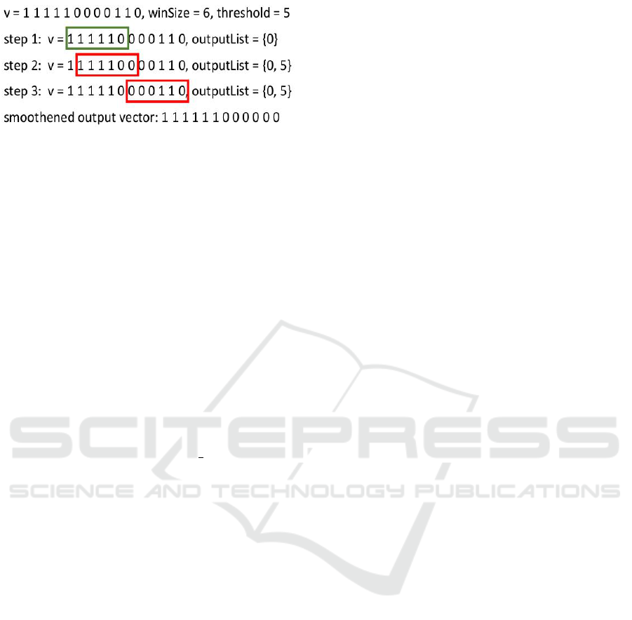
Figure 2: An example of applying the sliding window algo-
rithm. v is the input vector, and the output smoothed vec-
tor is constructed from the outputList on the last line. The
Green (Red) rectangle shows a window for which the count
of 1s in the window exceeds (does not exceed) the thresh-
old.
catenation should always be done in the same order.
In our analysis, we have considered only the primary
directions (phases 2 and 6) while creating the concate-
nated vector f av, with phase 2 followed by phase 6.
This step concludes the first stage of processing the
ATSPM data. Thus far, we have summarized the split
failures and laid the foundation for further processing.
In the second stage, each pair of f av vectors is
compared and a distance matrix computed. The idea
is to quantify the similarity or dissimilarity of all pairs
of vectors that are being compared. The distance be-
tween two f av vectors is defined as the 1-norm of the
difference vector. A vector p-norm is defined as
k
x
k
p
= (
∑
i
| x
i
|
p
)
1
p
(1)
and the 1-norm is defined as
k
x
k
1
= (
∑
i
| x
i
|). (2)
For example, f av1 is {12,1,0,10} and f av2 is
{10,5,0,5} the difference vector can be f av1 −
f av2 = {2,−4, 0, 5} or f av2− f av1 = {−2,4,0,−5}.
In either case the 1-norm is 11. This quantity is then
normalized; by dividing it with the 1-norm of the
larger vector. In the example, 11/23 is the normal-
ized distance between the two f av vectors.
The distances between all pairs of f av vectors are
stored in a distance matrix. Thus, if there are 300
intersections which need to be studied for 7 days, then
there are 7 ×300 = 2100 f av vectors and the distance
matrix is of size 2100 × 2100. Note that the distances
in the matrix for any pair of intersections represents
the behavioral distance between the intersections and
not just the Euclidean distance between them.
Based on the distance matrix, a number of clus-
tering algorithms can be applied to cluster the simi-
larly performing intersections. These algorithms are
explained in detail as follows.
Spectral Clustering. The use of spectral clustering
is quite appropriate here, since the data points are
generally not compact and are not naturally clustered
within convex boundaries. Using the distance matrix
computed in the previous section, a graph Laplacian
is constructed as the first step. A Laplacian matrix, L,
for an undirected simple graph G with n vertices, is
an n × n matrix such that
L = D − A (3)
where D is the degree matrix and A is the adjacency
matrix. An eigenvalue problem is solved as the next
step and k eigenvectors are chosen that correspond to
the k lowest eigenvalues, to give the k cluster centers.
This algorithm requires the users to input the number
of clusters k and may perform sub optimally if the cor-
rect number of clusters is unknown. We used a spec-
tral implementation available in the Python toolkit
Scikit-Learn.
Affinity Propagation. Affinity propagation is a
clustering algorithm that does not require the user to
input the number of clusters. The algorithm takes a
distance matrix as input and all data points are con-
sidered simultaneously as potential exemplars. Affin-
ity propagation works by the exchange of real-valued
messages between data points until a high-quality set
of exemplars emerges and corresponding clusters are
derived. For our model, we used the affinity prop-
agation implementation available in the Scikit-Learn
library in Python.
Spatial Information. Sometimes the intersections
belonging to a cluster are spread over geographic re-
gions over 10 miles apart. While these intersections
may be behaving similarly, there is no real value in
having such distant intersections in the same cluster if
we wanted to modify signal plans, for example. So, in
our work, we often do a second round of processing
where we split a cluster of intersections into multi-
ple disjoint clusters based on a geographical indicator
like primary road names, distance or the hop distance
between the intersections.
3.3 Categorization of Intersections
We use split failures in conjunction with the ratio of
arrivals on red to arrivals on green (AoR/AoG), to cat-
egorize the signals into four broad categories.
1. Low split failures, Low AoR/AoG: Low Demand
but potential for timing improvement.
2. Low split failures, High AoR/AoG: Well timed
and utilized intersection.
VEHITS 2019 - 5th International Conference on Vehicle Technology and Intelligent Transport Systems
142

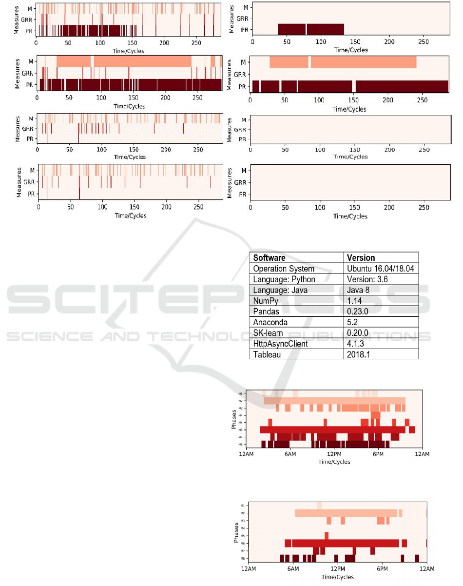
Figure 3: Multiple MOE’s for a Single Intersection Before and After Smoothing.
3. High split failures, Low AoR/AoG: High Demand
and Potential timing optimization.
4. High split failures, High AoR/AoG: Capacity
problem.
The thresholds that are used to separate low vs
high split failures and AoR/G, are intended to be flex-
ible based on feedback from local traffic engineers.
The same intersection will likely exhibit multiple be-
havioral modes depending on the time of a day or the
day of a week. For example, at night and early morn-
ing some of the intersections will have no demand,
where as during peak hours these same intersections
may see capacity issues.
4 EXPERIMENTS AND RESULTS
In this section, we first detail the software platform
used for performing data analytics on ATSPM data.
The data we used in this paper was provided by
Florida Department of Transportation (FDOT), Dis-
trict 5. Our implementation is based in Python, and
we used libraries such as NumPy, Scikit-Learn and
Pandas and Tableau (R) for visualization . Details are
provided in Figure 4.
We used the ATSPM data received from more
than 300 controllers in Seminole County, Orlando,
Florida. Figures 5 and 6 show split failures reported
at one intersection on a weekday vs the weekend re-
spectively. The background color represents no split
failures, while the darker foreground colors represent
Figure 4: Software stack used for our work.
Figure 5: An example of Split-failures after smoothing on a
Weekday.
Figure 6: An example of Split-failures for Intersection ID
1045, after smoothing, during the Weekend.
Analyzing Traffic Signal Performance Measures to Automatically Classify Signalized Intersections
143

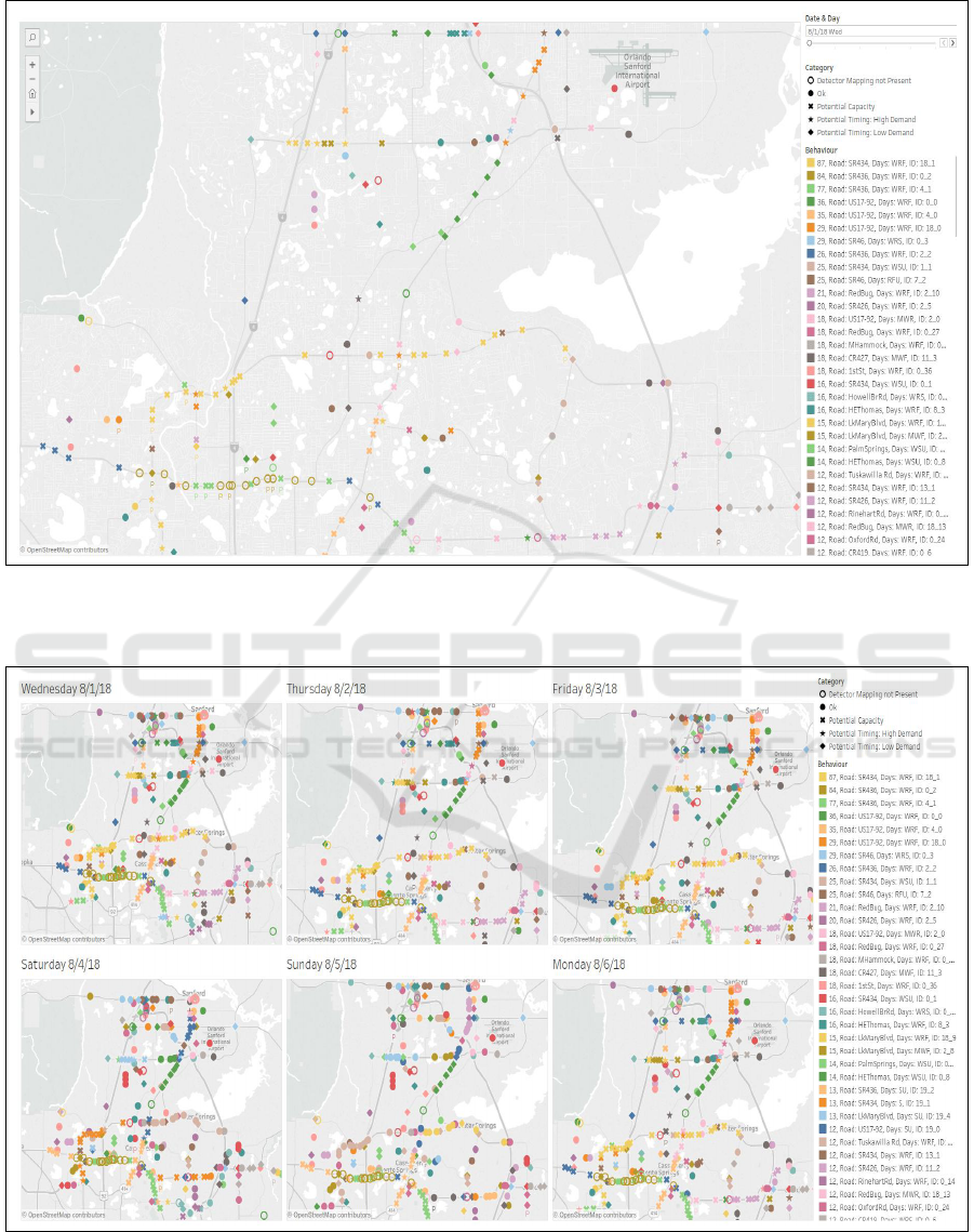
Figure 7: Dashboard showing the clustering & classification results for a single day. The results show that intersections on the
same corridor demonstrate similar behavior throughout the day. These correspond to a spatio-temporal cluster derived using
the approach described in the paper.
Figure 8: Multi-day Tableau dashboard allows for comparison of clustering results across days and highlights temporal
patterns in intersection behaviour. The behaviour on weekdays is contrasted with the weekend behaviour.
VEHITS 2019 - 5th International Conference on Vehicle Technology and Intelligent Transport Systems
144

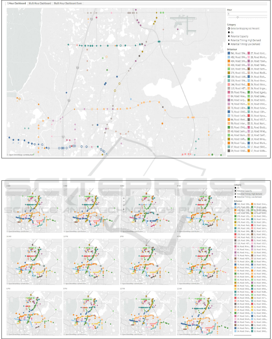
Figure 9: Hourly dashboard highlighting spatially confined clusters for a single hour. The spatio-temporal cluster membership
is highlighted by the color.
Figure 10: The multi-hourly dashboard highlighting the temporal recurrence of clusters during the day. Specifically, the early
morning/late night behaviour can be compared and contrasted with the daytime behaviour.
split failures, with each color representing a phase. As
expected, we observe a high volume of failures on the
weekdays when compared with weekends.
Figures 7, 8, 9 and 10 show a snapshot of a visu-
Analyzing Traffic Signal Performance Measures to Automatically Classify Signalized Intersections
145

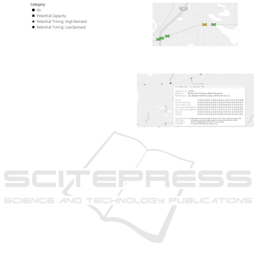
Figure 11: A magnified version of the category legend.
alization built in Tableau to present our results. The
intersections with similar performance are clustered
together using the same color. Recall that we use de-
mand based split failures along the major phases (2
and 6) for clustering the intersections. Further, each
intersection is categorized into one of four categories
as described in Section 3.3. These categories are rep-
resented by different shapes in the category legend,
which is shown separately in Figure 11.
For each cluster, the behavior legend presents the
corresponding color, the number of members, the
name of the road where the members may be found,
the days of the week that the cluster was observed and
finally a unique cluster identifier that was generated
by our algorithm. By hovering over each intersection
(Figure 13) we get more information, such as the sig-
nal ID, the number of split failures that happened on
an hourly basis for the major approaches, the number
of arrivals on red and green and the number of pedes-
trian actuation that happened along the minor phases
(4 and 8) which in turn affected the traffic flow on
the major phases. Figure 7 shows a dashboard of the
results on a single day, Figure 8 shows a dashboard
of the clustering results for each of the different days
studied.
The key findings from Figures 7 and 8 are summa-
rized as follows. We observed that behavioral clus-
tering of signalized intersections resulted in spatial
and temporal patterns in the results. In particular,
many signals on the same corridor get grouped to-
gether showing they behaved similarly during the day.
The clustering results in Figure 8 show that for many
intersections, the performance is similar during week-
days and different for the weekend. According to our
model most of the intersections perform well on Sun-
day, while these very same intersections have poten-
tial capacity issues on weekdays.
Further, we found that our clustering is in agree-
ment with categorization done in post processing. For
example, clusters predominantly contain intersections
which have either high or low split failures (high
or low demand categories, respectively) but rarely
both. Moreover, our clustering technique is sensi-
tive enough to capture granular differences between
the observed behavior of intersections. Some (spa-
tially confined) clusters of good intersections occur
only on weekends whereas some exist throughout the
Figure 12: An example where an intersection behaved dif-
ferently than the rest of the intersections on the same corri-
dor.
Figure 13: An example where phase 2 of Signal ID 1330
might have detection issues.
period that we analyzed. The latter are comprised of
intersections that are in the regions with low demand
and hence demonstrate similar behavior throughout
the week.
Figure 10 shows our bi-hourly dashboard. Here
we observe the similar behavioral patterns at late
night/early morning versus another set of patterns
during the daytime. Figure 11 shows a magnified ver-
sion of the categories legend of ease of reference.
Apart from highlighting potential behavioral pat-
terns of the intersections, our clustering mechanism
is also useful in highlighting problems at certain in-
tersections in a corridor. These problematic con-
trollers/detectors will usually present themselves as a
different cluster (hence are easily identifiable by the
color differential) in a corridor. Figure 12 shows such
an example where the gold intersection reports Split
Failures throughout the day on weekdays including
in the early hours between 12AM - 6AM. The inter-
sections in the green cluster Max-out between 6AM
and 9PM, on weekdays. Thus, the gold intersection
behaves differently from the rest of the intersections
and consequently is clustered separately.
Figure 13 shows an example where a starred inter-
section appears in an artery. The pop up in this figure
has data about the starred intersection. Here, we find
that split failures for the phase 2 are all zeros which is
odd because the intersections to the left and right of
this intersection has capacity issues on both the direc-
tions 2 and 6.
Figure 14 shows another example where two ad-
jacent signals belong to different clusters because of
VEHITS 2019 - 5th International Conference on Vehicle Technology and Intelligent Transport Systems
146

Figure 14: An example where two adjacent signals belong
to different clusters because they register slightly different
demand patterns.
slight differences in behavior, namely that while one
registers high demands till 8pm, the other registers de-
mands till 9pm on weekdays. This example demon-
strates that our clustering technique is sensitive to this
level of granularity. Thus our clustering approach can
be used to understand key behaviors in a grid or net-
work of signalized intersections and hence to improve
the deployed policy. It can also be used to understand
the hours or days for which the traffic patterns are
similar and the time periods for which their might be
some problems.
5 CONCLUSIONS
We developed a data driven approach to process high
resolution (ATSPM) data obtained from traffic con-
trollers. As part of the process, we use split failures
as an MOE and developed algorithms to characterize
the performance of an intersection. We used cluster-
ing as the method of choice for primary data process-
ing. This enabled us to group together signals exhibit-
ing similar behavior. As a result, we highlight signals
that do not belong to the group, but are part of the
same arterial network. Thus, the approach automati-
cally draws attention to signals that need attention in
terms of adjusting the timing plan or fixing of detec-
tor errors. We use a simple classifier to further clas-
sify the signals based on whether they cater to high
or low demand (recorded split failures) and high or
low utilization of green time (based on Arrivals on
Red/Green Ratios).
We visualized the results obtained by analyzing
real data from Florida. Thus, our approach acts as a
decision support system for traffic engineers and traf-
fic managers and informs them about the current per-
formance of the signalized intersection in a region.
The results can be used to easily identify problem-
atic signalized intersections in a proactive manner.
Our overall approach can be further enhanced by effi-
ciently compacting key signal measures in a network
(or region) along both spatial and temporal dimen-
sions.
ACKNOWLEDGEMENTS
The work was supported in part by Florida Depart-
ment of transportation. The opinions, findings and
conclusions expressed in this publication are those of
the author(s) and not necessarily those of the Florida
Department of Transportation or the U.S. Department
of Transportation
REFERENCES
Amini, S., Gerostathopoulos, I., and Prehofer, C. (2017).
Big data analytics architecture for real-time traffic
control. In 2017 5th IEEE International Conference
on Models and Technologies for Intelligent Trans-
portation Systems (MT-ITS), pages 710–715.
Day, C., Bullock, D., Li, H., Remias, S., Hainen, A.,
Freije, R., Stevens, A., Sturdevant, J., and Brennan,
T. (2014). Performance Measures for Traffic Signal
Systems: An Outcome-Oriented Approach.
Horvitz, E., Apacible, J., Sarin, R., and Liao, L. (July,
2005). Prediction, expectation, and surprise: Meth-
ods, designs, and study of a deployed traffic forecast-
ing service. 21st Conference on Uncertainty in Artifi-
cial Intelligence.
Huang, T., Poddar, S., Aguilar, C., Sharma, A., Smaglik,
E., Kothuri, S., and Koonce, P. (2018). Building intel-
ligence in automated traffic signal performance mea-
sures with advanced data analytics. Transportation
Research Record, 0(0):0361198118791380.
Li, H., M. Richardson, L., Day, C., Howard, J., and Bul-
lock, D. (2017). Scalable dashboard for identify-
ing split failures and heuristic for reallocating split
times. Transportation Research Record: Journal of
the Transportation Research Board, 2620:83–95.
Radivojevic, D. and Stevanovic, A. (2017). Framework
for quantitative annual evaluation of traffic signal sys-
tems. Traffic Signal Systems: Volume 1.
Smaglik, E. J., Bullock, D. M., Gettman, D., Day, C. M.,
and Premachandra, H. (2011). Comparison of alter-
native real-time performance measures for measuring
signal phase utilization and identifying oversaturation.
Transportation Research Record, 2259(1):123–131.
UDOT (2017). Udot automated traffic signal performance
measures - automated traffic signal performance met-
rics. https://udottraffic.utah.gov/atspm/. (Accessed on
12/26/2018).
US Department of Transportation, F. H. A. (2008).
Traffic signal timing manual. https://ops.fhwa.dot.
gov/publications/fhwahop08024/index.htm#toc. (Ac-
cessed on 12/26/2018).
US Department of Transportation, F. H. A. (2013). Mea-
sures of effectiveness and validation guidance for
adaptive signal control technologies. https://ops.fhwa.
dot.gov/publications/fhwahop13031/index.htm#toc.
(Accessed on 12/26/2018).
Wemegah, T. D. and Zhu, S. (2017). Big data challenges
in transportation: A case study of traffic volume count
from massive radio frequency identification(rfid) data.
In 2017 International Conference on the Frontiers and
Advances in Data Science (FADS), pages 58–63.
Analyzing Traffic Signal Performance Measures to Automatically Classify Signalized Intersections
147