A Computationally Efficient MPC for Green Light Optimal Speed
Advisory of Highly Automated Vehicles
Stephan Uebel
1
, Steffen Kutter
1
, Kevin Hipp
2
and Frank Schr
¨
odel
2
1
Chair of Vehicle Mechatronics, Technische Universit
¨
at Dresden, 01062 Dresden, Germany
2
Development Center Chemnitz/Stollberg, IAV GmbH, 09366 Stollberg, Germany
Keywords:
Optimal Control, Sequential Quadratic Program, Velocity Control, Model Predictive Control, Green Light
Optimal Speed Advisory, Highly Automated Driving, V2X.
Abstract:
The current study introduces an approach for energy efficient longitudinal vehicle guidance. The key idea is to
utilize a model predictive control (MPC) for the longitudinal vehicle dynamics which explicitly considers the
current and the predicted states of multiple traffic lights ahead. Consequently, the vehicle can drive in urban
situations much more energy efficient, which can be used to enlarge the range of electric vehicles or save
fuel while additionally improving travel time. Modern traffic lights are equipped with transmitters that send
information about their actual and upcoming system states. Additionally, traffic lights connected to a traffic
control center can broadcast their future signal phases to vehicles many kilometers ahead. This information
may be used to adapt the vehicle speed so that engine operation points are optimal and stops can be avoided.
These kind of algorithms are referred to as green light optimal speed advisory. This work presents a novel
online capable MPC approach that uses a sequential quadratic program to solve the respective optimal control
problem. This approach is implemented in a framework introduced as well which allows driving tests in a real
vehicle.
1 INTRODUCTION
The term green light optimal speed advisory
(GLOSA) comprises all procedures for approaching
traffic lights with vehicles in an optimal way by eval-
uating known or predicted information (traffic light
phases). Corresponding assistance systems for pas-
senger car drivers are well studied (Schuricht et al.,
2011) and already available as prototypes today or
are even in regular operation in trams (Gassel et al.,
2012).
In order to overcome the computational burden
of the underlying optimal control problem, typically
simplified vehicle models and only few traffic light
segments and phases (Erdmann, 2013) are taken into
account or sub-optimal, not online capable methods
like genetic algorithms (Seredynski et al., 2013) are
utilized.
A major drawback of the implementation in form
of a driver assistance system is the inclusion of the
human driver as the overall controller in the system,
since on the one hand there is an additional distraction
from the primary driving task (safety) and on the other
hand the driver’s control performance (accuracy and
speed) is poorer than technical systems.
With increasing vehicle automation the task of
optimally choosing the vehicle velocity with respect
to comfort, energy consumption and driving time is
therefore handed over to the highly automated driv-
ing system (HAD). The HAD combines both lateral
and longitudinal vehicle control with respect to the
detected surrounding traffic situation and the planned
path of the ego vehicle.
The current study focuses on optimizing the vehi-
cle velocity in a HAD. Optimal velocity control has
already been applied to conventional vehicles. For in-
stance, an early implementation of real-time optimal
velocity control using dynamic programming (DP)
(Bellman, 1954) was presented by Porsche, called
ACC InnoDrive (Radke, 2013). Other approaches us-
ing DP concentrate on controlling velocity on short-
range trips, e.g. the distance between two traffic lights
(Dib et al., 2011; Themann et al., 2014). Using DP
for both, velocity control and gear shifting of conven-
tional trucks, has been proposed in (Hellstr
¨
om et al.,
2009; Hellstr
¨
om et al., 2010). Furthermore, DP is
used for optimal velocity control of truck platoons
(B
¨
uhler, 2013), but there, for the sake of compu-
444
Uebel, S., Kutter, S., Hipp, K. and Schrödel, F.
A Computationally Efficient MPC for Green Light Optimal Speed Advisory of Highly Automated Vehicles.
DOI: 10.5220/0007717304440451
In Proceedings of the 5th International Conference on Vehicle Technology and Intelligent Transport Systems (VEHITS 2019), pages 444-451
ISBN: 978-989-758-374-2
Copyright
c
 2019 by SCITEPRESS – Science and Technology Publications, Lda. All rights reserved

tational efficiency, gear, internal combustion engine
(ICE) on/off and travel time are removed from the
state vector, and the engine model is reduced to a
simple constant efficiency. Besides DP, other meth-
ods are examined for velocity control of conventional
vehicles. For instance, quadratic programming (QP)
(Boyd, 2004) has been proposed by (Gonsrang and
Kasper, 2015). Early research calculating the optimal
velocity of a conventional vehicle with Pontryagin’s
maximum principle (PMP) (Pontryagin et al., 1962)
was done by (Schwarzkopf and Leipnik, 1977). A
combination of QP and DP has been applied by (Mur-
govski et al., 2016) for optimal velocity control and
gear selection for a platoon of conventional vehicles.
Even the complex problem of computing the optimal
velocity of hybrid electric vehicle is solved by the au-
thors of (Uebel et al., 2018).
In contrast to the previous approaches mentioned,
this paper presents a novel algorithm combining op-
timal longitudinal control and GLOSA for multiple
traffic lights and phases into one, online capable con-
trol structure for a HAD. The algorithm uses a se-
quential quadratic program (SQP) (Mikosch et al.,
2006, p. 529 ff.) to find the optimal solution. The
close to optimal solution quality of this approach for
a more complex problem is shown in (Uebel, 2018),
by comparing the obtained results with the reference
solution, calculated with DP on a high performance
cluster at TU Dresden with over 8 months calculation
time. In result with assuming no costs for changing
gear, there is no deviation between the solutions but
the computational effort can be reduced to a millionth.
A case study for an implementation of the approach in
a Volkswagen Golf passenger car is presented which
shows the capability of the algorithm to compute the
optimal trajectories for the velocity implemented at an
online platform under real world driving conditions.
This paper is organized as follows. Section 2 in-
troduces all model equations leading to the descrip-
tion of the discrete optimal control problem (OCP).
Section 3 describes model abstractions that reduce the
computation time for the SQP. Afterwards, it is shown
how the SQP is used to solve the GLOSA problem.
Finally, a case study is performed and discussed.
2 PROBLEM DESCRIPTION
In this section, the GLOSA problem is formulated.
First a vehicle model is introduced which is used to
derive an OCP afterwards.
2.1 Vehicle Model
The powertrain of the model includes an internal com-
bustion engine (ICE) that converts chemical fuel en-
ergy to mechanical propulsion energy. The rotational
speed of the ICE
ω(v, g) =
v
r
γ(g) (1)
depends on the longitudinal vehicle velocity v, the dy-
namic rolling radius of the wheels r and the gear ratio
γ(g). Note, that g is not a control signal here because
the gear yielding the lowest fuel consumption is se-
lected at any instant (cf. 3.1).
The control signals are the ICE force F
E
= T
E
/r
and the mechanical brake force F
B
. They are gathered
in the vector of inputs
u = (F
E
,F
B
). (2)
The force F
E
is translated by the gearbox to a
wheel force. The gearbox has an efficiency η
g
that
determines its dissipative force
F
T,d
(u) =
(
F
E
(η
g
− 1)/η
g
, for F
E
≤ 0
F
E
(1 − η
g
), for F
E
> 0
(3)
which counteracts the wheel force. The brake and the
driving resistance due to inertia, air drag and road
slope cause further counteracting forces. Accord-
ingly, the balance of forces at the wheel is
mv
dv
ds
+ c
a
v
2
+ c
α
+ F
B
= (F
E
− F
T,d
(u))γ(g),
∀s ∈ [s
0
,s
f
],
(4)
where m is the vehicle mass, c
a
is a constant for the air
drag and c
α
a slope-dependent disturbance that com-
bines the rolling resistance and the force due to road
gradient. The balance is formulated in a space coor-
dinate s which denotes the travelled distance starting
from an initial position s
0
to a final position s
f
. The
term vdv/ds in (4) derives directly from the time to
space transformation
dv
dt
= v
dv
ds
. (5)
Note that, for brevity, the dependency on s is not dis-
played. All states and control signals and some coef-
ficients in this paper depend on s. Constants that do
not depend on s are displayed in upright letters. For
instance in (4), c
a
does not depend on s while c
α
does.
It can be noticed that the state dynamics in (4) are
nonlinear. A straightforward way to remove nonlin-
earity, without introducing approximations, is to per-
form a variable change, where kinetic energy
E
V
=
1
2
mv
2
(6)
A Computationally Efficient MPC for Green Light Optimal Speed Advisory of Highly Automated Vehicles
445

is used as system state instead of longitudinal veloc-
ity. In space domain, the derivative of vehicle energy
transforms into
∂E
V
∂s
= E
0
V
=
1
2
m
dv
2
ds
= mv
dv
ds
= mvv
0
, (7)
where the prime symbol (
0
) is used as a shorthand
notation for the first derivative with respect to s. As a
consequence of (7), (4) can be written as
E
0
V
= f
V
(u,E
V
) =
(F
E
− F
T,d
(u))γ(g) − F
B
− 2c
a
E
V
/m − c
α
∈ m[a
min
,a
max
],
(8)
which gives the state differential equation of the ki-
netic energy f
V
that is limited by the minimum ac-
celeration a
min
and the maximum acceleration a
max
,
introduced to ensure driver comfort.
Since the problem is formulated in space coordi-
nates, the travel time t becomes a system state. Its
dynamics are expressed by
t
0
= 1/v = 1/
p
2E
V
/m = f
t
(E
V
). (9)
The system states are gathered in the complete state
vector
x = (x
c
,x
d
). (10)
2.2 Problem Formulation
This section formulates the OCP in discrete space us-
ing the previously introduced model, where k is the
discrete index for the position. The same symbols that
were used in the continuous time representation, are
used in this section to denote discrete signals.
The main objective is to minimize the monetary
costs for a given route, subject to state and control
constraints. The costs are expressed as the consumed
fuel energy over the horizon multiplied by the respec-
tive price κ
E
. The fuel energy is the product of the
sample length ∆s(k) and the sum of F
E
and the dissi-
pative ICE force F
E,d
(F
E
,x), which is provided by a
lookup table.
The ensued OCP,
minimizeJ (u(k), x(k),k) (11a)
= κ
E
N
k
∑
k=1
(F
E
(k) + F
E,d
(F
E
(k), x(k))γ(g(k))∆s(k)
subject to
x(k + 1) = x(k) + f(u(k),x(k),k)∆s(k), (11b)
x(1) = x
0
, (11c)
f
V
(k) ∈ m[a
min
,a
max
], (11d)
x ∈ [x
min
(k), x
max
(k)], (11e)
u ∈ [u
min
(x(k)),u
max
(x(k))], (11f)
contains the function
f(u(k),x(k),k) = ( f
V
(k), f
t
(k)) (12)
which combines the state dynamics of the states. The
initial state conditions are given by the vectors x
0
and
the state space of the OCP (11) is bounded by lower
(x
min
(k)) and upper (x
max
(k)) limits.
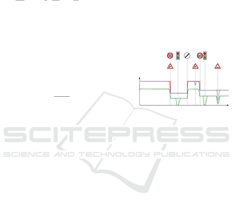
2.3 Velocity and Time Boundaries
An example for the boundaries on kinetic energy de-
pitcs Figure 1, where the upper limit is obtained by
100
80
60
40
20
0 1 2 3 4 5 6 7 8
Position (km)
Velocity (km/h)
Figure 1: Boundaries to the velocity (kinetic energy). The
red line represents the legal speed limit, while the blue line
depicts limits due to a maximum cornering speed. The
green line is the lower speed limit.
considering legal speed limits (red line). Addition-
ally, demands on comfort (Bellem et al., 2016), (Rey-
mond et al., 2001), (Scherer et al., 2015) as well
as existing standards (International Organization for
Standardization, 2009) limit the longitudinal and lat-
eral acceleration, which lowers the maximum veloc-
ity (blue line). The lower bound on the velocity is
obtained by subtracting a constant value from the up-
per speed limit (green trajectory). This value is in-
fluenced by the surrounding traffic, e.g. if the value
is selected too high, the vehicle might be an obstacle.
However, when approaching intersections and traffic
lights lower velocities are accepted (green semicolon
velocity) to enable a stop of the vehicle.
It can be understood that the time is bounded by
the bounds on E
V
. For example, the shortest time to
a position can be derived following the upper limit
on E
V
(highest velocity). Additionally, the time is
bounded by the timing of the traffic lights phases,
which is illustrated in the upper plots of Figure 4 and
5 in the results section.
2.4 ACC and Stop-line Functions
Solving problem (11) purely in a MPC is not suf-
ficient to implement a longitudinal velocity control
VEHITS 2019 - 5th International Conference on Vehicle Technology and Intelligent Transport Systems
446

under real conditions (cf. Section 4). For example
slower vehicles driving ahead on the same lane are
neglected by the OCP. However, the solution of the
OCP (11) can be used as a set velocity for a controller
that works as a typical ACC when approaching a ve-
hicle or can assure stopping at the stop line of a red
traffic light.
Therefore, an algorithm solving (11) is utilized for
the calculation of the optimal velocity with a long pre-
diction horizon and explicit consideration of traffic
lights. The computed target set is used for a shorter
horizon by a lower level which contains an ACC and
a stop-line approaching function.
A modular control design realizes both functions,
which is a straightforward way of changing between
different control modes. Following, three common
modes are listed.
• Speed-based longitudinal dynamic control: The
controller follows a given velocity which is ob-
tained from the OCP algorithm. The controller
structure corresponds to a conventional cruise
control.
• Object-based longitudinal dynamic control: The
controller uses sensor data to take vehicles driving
ahead and other objects into account. The con-
troller structure corresponds to a classic ACC.
• Trajectory-based longitudinal dynamic control:
This mode realizes an accurate longitudinal dy-
namic trajectory tracking without imposing an ad-
ditional dynamic on the system. In this controller
mode, high requirements with regard to follow a
given velocity trajectory (e.g. to brake at a stop
line) must be realized in order to ensure driving
comfort and safety to other road users.
In order to react to slower road participants driv-
ing ahead, the ACC reduces the desired speed, com-
puted by the OCP algorithm. In detail, the distance
to the vehicle ahead is controlled in an outer-control
loop, which results in a new set speed for the vehicle,
while the desired speed is controlled within the inner-
control loop. In the current set up of the test vehicle,
an acceleration instead of a velocity interface is used
for the longitudinal guidance. Therefore, the chosen
acceleration set point is transmitted to the acceleration
controller, which computes the corespondent engine
and brake torques.
Because of a higher update time the OCP algo-
rithm cannot guarantee a stop at the precise position
of the stop line. Due to this a trajectory-based longi-
tudinal controller is used for stopping the vehicle. It
activates if the velocity drops below a specific vehicle
speed (e.g. 10 km/h) and uses an extra front camera
and corresponding algorithms to determine the cor-
rect position of the stop line. This position is used to
calculate a precise breaking trajectory.
3 GLOSA COMPUTATION
It is not straightforward to regard a set of time con-
straints which are imposed by the phases of a traffic
light with the OCP formulated in the previous sec-
tion. The reason is that the OCP formulation (11)
allows only one value for the lower and one for the
upper time boundary (cf. (11e)) at each instant (po-
sition) while several lower and upper boundaries are
necessary to consider the phases of the traffic lights.
Consequently, to find the optimal solution for the
GLOSA problem the OCP has to be computed sev-
eral time with different values for the time constraints
at each computation. Consequently, in order to solve
the GLOSA problem online, this section formulates
the OCP as an SQP scheme, for which there are com-
putationally efficient solvers.
3.1 Approximated Objective
Following, several steps are proposed to adapt the
model in order to incorporate a fast solver
1
that de-
creases the computational demand, including abstrac-
tion of the engine transmission unit and a conservative
QP modeling for an SQP scheme.
As stated before gear shifts are assumed to be in-
stantaneous and the gears are optimized in advance,
by preselecting gears that minimize fuel consumption
when the ICE is propelling the vehicle. Thus, instead
of investigating the fuel consumption map on the en-
gine side, a corresponding fuel consumption map is
generated for the engine transmission unit which pro-
vides the force
˜
F
E,W
to the wheel. As there is a redun-
dancy, in the sense that different gears may provide
the same force-speed points, it is possible to chose op-
timal gears that minimize fuel consumption for each
operating point. The obtained fuel consumption map
is then approximated by the following analytic ex-
pression
˜
P
E
= ζ
0
+
p
˜
E
V
(ζ
1
+ζ
2
˜
E
V
+ζ
3
˜
F
E,W
+ζ
4
˜
F
2
E,W
+ζ
5
˜
E
2
V
).
(13)
The over-line symbol tilde (
˜
{·}) is used to denote ap-
proximated signals of the SQP.
The objective of the SQP is to minimize the mon-
etary costs
1
ECOS presented in (Domahidi et al., 2013) is used.
A Computationally Efficient MPC for Green Light Optimal Speed Advisory of Highly Automated Vehicles
447

J(
˜
t,
˜
E
V
,
˜
F
E,W
,
˜
E
S
) = κ
E
Z
s
f
s
0
˜
P
E
v
ds
= κ
S
(
˜
E
S0
−
˜
E
S
(s
f
)) + κ
E
ζ
0
Z
s
f
s
0
1
v
ds +κ
E
ζ
1
Z
s
f
s
0
ds
+ κ
E
r
m
2
Z
s
f
s
0

ζ
2
˜
E
V
+ ζ
3
˜
F
E,W
+ ζ
4
˜
F
2
E,W
+ ζ
5
˜
E
2
V

ds
= κ
S
(
˜
E
S0
−
˜
E
S
(s
f
)) + κ
E
ζ
0
(
˜
t(s
f
) −
˜
t
0
) + κ
E
ζ
1
(s
f
− s
0
)
+ κ
E
r
m
2
Z
s
f
s
0

ζ
2
˜
E
V
+ ζ
3
˜
F
E,W
+ ζ
4
˜
F
2
E,W
+ ζ
5
˜
E
2
V

ds
(14)
which is a quadratic convex function. The terms in-
cluding t
0
as well as the term multiplied by ζ
1
are con-
stants that can be removed from the objective, without
affecting the optimal solution. The objective can then
be written in a discrete form, as discussed in Section
2.2.
3.2 Approximated Constraints
The maximum force that the engine-transmission unit
can deliver is illustrated in Figure 2. It can be ob-
served that the force limit is a highly nonlinear and
partly discrete function. To remove the need for in-
teger decisions, a piecewise nonlinear inner approxi-
mation is performed, of the form
˜
F
E,Wmax
= min


ζ
W,1
+ ζ
W,2
˜
E
V
,
ζ
W,3
,
ζ
W,4
+ ζ
W,5
/
p
˜
E
V


. (15)
The inner approximation ensures that a solution ob-
tained by solving the approximated problem is feasi-
ble also in the original problem. It can be observed
in Figure 2 that the force limit, left of the peak point,
is a concave function. A concave function can be ap-
proximated with a negligible error by expressing it as
the minimum of sufficiently many affine pieces. Only
two such pieces have been used here (the first two in
(15)). Finally, the last, nonlinear piece in (15) is cho-
sen to capture the power limit of the engine, as it is an
alternative expression of an inverse speed relation.
0 50 100 150
v (km/h)
0
20
40
60
80
100
Normalized
˜
F
E,Wmax
(%)
0 0.5 1 1.5 2
E
v
(MJ)
Original
Approximated
Figure 2: Approximated maximum force of the engine-
transmission unit over velocity (left) and over kinetic energy
(right) compared to the original model.
The nonlinear time dynamics,
˜
t
0
= 1/
q
2
˜
E
V
/m (16)
cannot be expressed as a quadratic function and are
therefore approximated using a reference kinetic en-
ergy,
ˆ
˜
E
V
, about which linearizations are performed;
further discussed below.
The obtained optimization problem has now linear
dynamics
˜
E
0
S
= −
˜
F
S
(17a)
˜
E
0
V
=
˜
F
E,W
−
˜
F
B
− 2c
a
˜
E
V
/m − c
α
(17b)
˜
t
0
= 1/
q
2
ˆ
˜
E
V
/m (17c)
but nonlinear and non-convex constraints, due to the
nonlinear term 1/
p
˜
E
V
in the force limits of the
engine-transmission, (15). Due to the sign of the co-
efficients multiplying 1/
p
˜
E
V
, it can be observed that
this term is convex. Therefore, linearizing it about the
reference trajectory
ˆ
˜
E
V
,
1/
p
˜
E
V
≈ f
lin
(
˜
E
V
,
ˆ
˜
E
V
) (18)
provides a convex inner approximation. This is the
final ingredient for developing a computationally effi-
cient SQP.
3.3 Approximated Problem
Formulation
By defining the state and control vectors as
˜
x = (
˜
E
V
,
˜
t),
˜
u = (
˜
F
E,W
,
˜
F
M,W
,
˜
F
B
) (19)
and by discretizing with, e.g., zero-order hold, the re-
sulting QP solved in each iteration of the SQP can be
summarized as
minimizeJ(
˜
x(
˜
k),
˜
u(
˜
k)) + Q(
˜
x(
˜
k),
˜
u(
˜
k)) (20a)
subject to
˜
x(
˜
k + 1) = A
A
A(
˜
k)
˜
x(
˜
k) + B
B
B(
˜
k)
˜
u(
˜
k) + w(
˜
k) (20b)
C
C
C(
˜
k)
˜
x(
˜
k) + D
D
D(
˜
k)
˜
u(
˜
k) ≤ b(
˜
k) (20c)
˜
x(
˜
k) ∈ [
˜
x
min
(
˜
k),
˜
x
max
(
˜
k)] (20d)
˜
u(
˜
k) ∈ [
˜
u
min
(
˜
k),
˜
u
max
(
˜
k)] (20e)
˜
x(0) =
˜
x
0
,
˜
t(N
k
) <=
˜
t
f
(20f)
(20g)
where the matrices A
A
A, B
B
B, C
C
C, D
D
D and the vectors w, b,
˜
x
min
,
˜
x
max
, can be found from eqs. (15) and (17). Note
that these matrices and vectors depend on
˜
k since the
slope as well as the boundaries on
˜
E
V
and the
˜
t as
well as the approximation of t
0
depend on the posi-
tion. The distance between two samples
˜
k might be
VEHITS 2019 - 5th International Conference on Vehicle Technology and Intelligent Transport Systems
448

varying depending on the boundaries on
˜
E
V
, i.e. at
high velocities the sampling can be sparser.
The term Q in the objective is a standard term in
the SQP framework that provides additional search
direction towards the optimal solution that also min-
imizes the linearization error. It includes Hessian of
the Lagrangian and Jacobian of the objective function,
with respect to
˜
E
V
. For further details, see (Mikosch
et al., 2006). After each QP iteration, the trajectory
about which the problem is linearized (
ˆ
˜
E
V
) is updated
by moving towards the direction of the current opti-
mal solution. Thus,
ˆ
˜
E
V
is updated as
ˆ
˜
E
i+1
V
=
ˆ
˜
E
i
V
+ ξ(
˜
E
i∗
V
−
ˆ
˜
E
i
V
) (21)
where i is the current iteration, ∗ is the optimal so-
lution in the current iteration and ξ is the step size
that regulates the convergence rate. A high step size,
ξ = 1, has been chosen for this problem. The initial
trajectory
ˆ
˜
E
1
V
is selected as the mean between the up-
per and lower velocity boundaries.
4 CASE STUDY
This section presents a case study of the GLOSA ap-
proach. Before results for two different traffic light
timings are shown, the test arrangement is presented.
4.1 Framework
The HAD framework depicted in Figure 3 consists of
three layers which is similar to classic robotic solu-
tions.
The first layer realizes the environment perception
with the main focus on object detection and predic-
tion as well as on lane detection and free space cal-
culation. The second layer consist of decision mak-
ing, including strategic, tactical and operational plan-
ing. The strategy module realizes route calculation
and abstract mission planning. It derives prioritized
missions and a route enhanced by abstract action re-
quests. Therefore, it optimizes the whole route of the
vehicle with respect to driving time, comfort and mis-
sion fulfillment.
The tactical module aims to generate optimal driv-
ing maneuver requests (e.g. lane change, lane keep-
ing, parking) in order to follow the strategic route
and actions. It continuously checks the driving state
against the target state (e.g. target speed and target
lane) and attempts to optimize the short term travel-
ing behavior.
The operational module supplies atomic driving
maneuvers such as lane keeping, lane change, etc.
This lowest decision level knows the feasibility of
each individual driving maneuver and tries to fulfill
the requirements of the tactical level by using path
planning algorithms. Below the decision layer, the
trajectory planing and lateral and longitudinal vehi-
cle dynamic controllers realize the detailed movement
planing and tracing task in side the third layer.
4.2 Vehicle
The test vehicle which is used in the current study, is
a VW Golf VII which is equipped with computation
hardware (a dSPACE MicroAutoBox II and an indus-
try PC).
4.3 Route
A test track near the airfield of the city of Dresden in
Saxony/Germany was selected which is about 6.6 km
long and equipped with four traffic lights. For future
real driving tests these traffic lights are equipped with
communication hardware in order to send the planned
traffic light phases to the test vehicle.
4.4 Results
The longitudinal control of the approach is evaluated
in two simulations: First, a simulation of the test track
is performed where measured traffic light timings are
used, to show the general capability of the algorithm
to find the optimal speed through green phases of sev-
eral traffic lights. For the second simulation the tim-
ing is changed, so the vehicle has to stop at the third
traffic light.
The results of the two simulations are shown in
the Figures 4 and 5, where the top plots shows the
timing of the traffic light phases over the position.
Additionally, the bound on the time derived from the
minimum velocity is shown by the dotted line. It can
be observed in both figures that following the mini-
mum velocity would cause driving through a red light
phase of the second traffic light. Due to this, the ap-
proach decreases the velocity yielding the one shown
with the time trajectory depicted with a solid line in
the upper plots.
The bottom plots show the associated velocity tra-
jectories with solid lines, as well. The planned bounds
on the velocity are shown with dotted lines. In or-
der to avoid driving through red light, the minimum
velocity has to be adapted which is done in the first
half of the route. However, adaption is only allowed
to about 60 % of the maximum velocity. Even with
adaption of the velocity it is not possible to reach a
A Computationally Efficient MPC for Green Light Optimal Speed Advisory of Highly Automated Vehicles
449

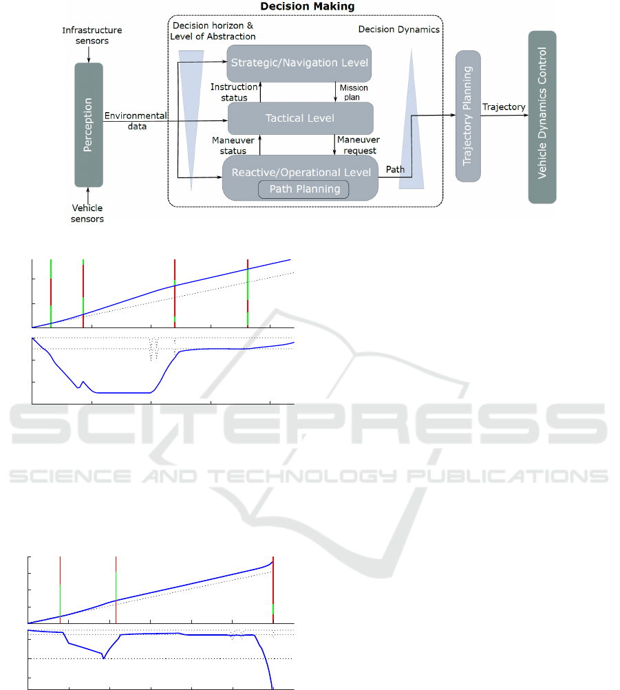
Figure 3: Functional Architecture for HAD System.
0
50
100
Time (s)
0 500 1000 1500 2000
Position (m)
40
50
60
70
Velocity(km/h)
Figure 4: Results of the first simulation. The top plot shows
the phase timing of the traffic lights and the time trajectory
yielded by the algorithm, while the bottom plot depicts the
associated velocity trajectory of the vehicle. The planned
lower state bound for the velocity (lower dotted line) is vio-
lated at some instances in order to reach the green phase of
the next traffic light.
0
20
40
60
80
Time (s)
0 200 400 600 800 1000 1200
Position (m)
20
40
60
Velocity (km/h)
Figure 5: Results of the second simulation where a stop at
the third traffic light is inevitable. In contrast to the first
simulation, the vehicle accelerates to the minimum velocity
before braking at the third traffic light.
green phase of the third traffic light in the second sim-
ulation shown in Figure 5. Consequently, the algo-
rithm accelerates to the minimum velocity and brakes
before the third traffic light. In order not be an obsta-
cle for other road participants, the algorithm is con-
figured to avoid a slow deceleration after the second
traffic light which would be energy efficient. The ma-
jor part of road users does not accept driving less than
the minimum velocity shown in Figures 4 and 5 even
when approaching a red light as we experienced in
real world testing.
5 CONCLUSIONS
The simulations show that the introduced novel MPC
algorithm for GLOSA which solves a set of OCPs
using an SQP scheme is suitable for real driving
tests. Performing these tests will be the next step.
Therefore, the algorithm is already successfully im-
plemented to the HAD framework presented in this
paper where it performed with a turnaround time of
about 0.2 s. The main challenge is to obtain a predic-
tion of the traffic light phase timings with a sufficient
horizon length since their signals are traffic-actuated.
ACKNOWLEDGEMENTS
The research shown here is related to the project
initiative ”Syncronized Mobility 2023” and part of
the projects ”REMAS”, ”SYNCAR” and ”Harmo-
nizeDD” which are publicly funded by the European
Union and the Federal Ministry of Transport and Dig-
ital Infrastructure in Germany. Additionally, the au-
thors would like to thank The Center for Information
Services and High Performance Computing (ZIH) at
Technische Universit
¨
at Dresden.
VEHITS 2019 - 5th International Conference on Vehicle Technology and Intelligent Transport Systems
450

REFERENCES
Bellem, H., Sch
¨
onenberg, T., Krems, J. F., and Schrauf, M.
(2016). Objective metrics of comfort: Developing a
driving style for highly automated vehicles. Trans-
portation Research Part F: Traffic Psychology and Be-
haviour, 41:45–54.
Bellman, R. (1954). The theory of dynamic program-
ming. Bulletin of the American Mathematical Society,
60(6):503–515.
Boyd, S. (2004). Convex optimization. Cambridge Univer-
sity Press, Cambridge, U.K.
B
¨
uhler, L. (2013). Fuel-Efficient Platooning of Heavy Duty
Vehicles through Road Topography Preview Informa-
tion. Master’s thesis, Automatic Control Laboratory -
KTH Royal Institute of Technology, Stockholm, Swe-
den.
Dib, W., Serrao, L., and Sciarretta, A. (2011). Optimal
control to minimize trip time and energy consump-
tion in electric vehicles. In 2011 IEEE Vehicle Power
and Propulsion Conference (VPPC), pages 1–8, Pis-
cataway, New Jersey, USA. Institute of Electrical and
Electronics Engineers (IEEE).
Domahidi, A., Chu, E., and Boyd, S. (2013). ECOS: An
SOCP Solver for Embedded Systems. In Proceed-
ings European Control Conference, pages 3071–3076,
Zurich, Switzerland.
Erdmann, J. (2013). Combining adaptive junction con-
trol with simultaneous Green-Light-Optimal-Speed-
Advisory. In 5th International Symposium on Wireless
Vehicular Communications (WiVeC), pages 1–5.
Gassel, C., Matschek, T., and Krimmling, J. (2012). Coop-
erative Traffic Signals for Energy Efficient Driving in
Tramway Systems. In Intelligent Transportation Soci-
ety of America, editor, 19
th
ITS World Congress.
Gonsrang, S. and Kasper, R. (2015). Optimization-based
Energy Management System for Pure Electric Vehi-
cles. In B
¨
aker, B. and Morawietz, L., editors, Energy
efficient vehicles 2015: Visions, trends and solutions
for energy efficient vehicle systems, volume 5, pages
100–110. TUDpress, Dresden, Germany.
Hellstr
¨
om, E.,
˚
Aslund, J., and Nielsen, L. (2010). Design
of an efficient algorithm for fuel-optimal look-ahead
control. Control Engineering Practice, 18(11):1318–
1327.
Hellstr
¨
om, E., Ivarsson, M.,
˚
Aslund, J., and Nielsen, L.
(2009). Look-ahead control for heavy trucks to min-
imize trip time and fuel consumption. Control Engi-
neering Practice, 17(2):245–254.
International Organization for Standardization (2009). ISO
22179:2009 - Intelligent transport systems - Full
speed range adaptive cruise control (FSRA) systems
- Performance requirements and test procedures: Per-
formance requirements and test procedures.
Mikosch, T. V., Wright Stephen J, and Nocedal Jorge
(2006). Numerical Optimization. Springer series in
operations research Numerical optimization. Springer,
New York, USA, 2 edition.
Murgovski, N., Egardt, B., and Nilsson, M. (2016). Co-
operative energy management of automated vehicles.
Control Engineering Practice, 57:84–98.
Pontryagin, L. S., Boltyanskii, V. G., Gamkrelidze, R. V.,
Mishchenko, E. F., and Pontr
ˆ
agin, L. S. (1962). The
Mathematical Theory of Optimal Processes. Inter-
science Publishers, New York, USA.
Radke, T. (2013). Energieoptimale L
¨
angsf
¨
uhrung von
Kraftfahrzeugen durch den Einsatz vorausschauender
Fahrstrategien, volume 19 of Karlsruher Schriften-
reihe Fahrzeugsystemtechnik. KIT Scientific Publish-
ing, Karlsruhe and Hannover, Germany.
Reymond, G., Kemeny, A., Droulez, J., and Berthoz, A.
(2001). Role of lateral acceleration in curve driving:
driver model and experiments on a real vehicle and a
driving simulator. Human factors, 43(3):483–495.
Scherer, S., Dettmann, A., Hartwich, F., Pech, T., Bullinger,
A. C., and Wanielik, G. (2015). How the driver wants
to be driven - Modelling driving styles in highly au-
tomated driving. Automatisiertes Fahren - Hype oder
mehr? In S
¨
ud, T., editor, 7. Tagung Fahrerassistenz,
M
¨
unchen.
Schuricht, P., Michler, O., and Baker, B. (2011). Efficiency-
increasing driver assistance at signalized intersections
using predictive traffic state estimation. In 14th Inter-
national IEEE Conference on Intelligent Transporta-
tion Systems (ITSC), 2011, pages 347–352, Washing-
ton, DC, USA.
Schwarzkopf, A. B. and Leipnik, R. B. (1977). Control of
highway vehicles for minimum fuel consumption over
varying terrain. Transportation Research, 11(4):279–
286.
Seredynski, M., Dorronsoro, B., and Khadraoui, D. (2013).
Comparison of Green Light Optimal Speed Advisory
approaches. In 16th International IEEE Conference
on Intelligent Transportation Systems (ITSC), pages
2187–2192, Piscataway, New Jersey, USA. Institute
of Electrical and Electronics Engineers (IEEE).
Themann, P., Zlocki, A., and Eckstein, L. (2014).
Energieeffiziente Fahrzeugl
¨
angsf
¨
uhrung durch
V2X-Kommunikation. ATZ - Automobiltechnische
Zeitschrift, 116(7-8):62–67.
Uebel, S. (2018). Ein im Hybridfahrzeug einset-
zbare Energiemanagementstrategie mit optimaler
L
¨
angsf
¨
uhrung. PhD thesis, Technische Universit
¨
at
Dresden, Dresden, Germany.
Uebel, S., Murgovski, N., Tempelhahn, C., and Baker, B.
(2018). Optimal Energy Management and Velocity
Control of Hybrid Electric Vehicles. IEEE Transac-
tions on Vehicular Technology, 67(1):327–337.
A Computationally Efficient MPC for Green Light Optimal Speed Advisory of Highly Automated Vehicles
451