
Turbulent Flow Modelling of a Jet in a Cross-Flow Stream:
Model and App
M. Tabatabaian
Department of Mechanical Engineering, British Columbia Institute of Technology, School of Energy,
3700 Willingdon Ave., Burnaby, BC, Canada
Keywords: Turbulent Flow, Jet Flow, Cross Flow, CFD, , Education-Aid App, COMSOL
®
.
Abstract: The flow of a jet stream entering a cross flow main stream is modelled along with introducing the related App.
The turbulent flow details are computed and validated against similar computational and experimental results.
For example, dimensionless streamwise and cross-streamwise velocity components, dimensionless turbulent
kinetic energy, and dissipation are shown in colour-expression figures, along with streamlines near the jet
entrance to the main stream flow. The results agree with those from the existing references. We used a custom
designed structured mesh for all models. Also, for democratization of the model applications a COMSOL®
model-based App is built and introduced
a
.
1 INTRODUCTION
The topic of turbulent flow modelling of a crossflow
jet is of interest, both for understanding of the flow
detail and industrial applications. This type of flow
occurs in many industrial and natural applications.
For instance, during landing and take-off of airplanes,
gas turbines, fuel injections, oil refinery piping, waste
discharge into reservoirs or atmosphere. In any of
these flow types turbulence occurs and enhances
mixing or, in general, the exchange of mass and
energy between the jet and the mainstream flows.
With the advances of computational fluid dynamics
(CFD) and practical availability of commercial CFD
software tools more industries are using models of
turbulent flows in their design process. COMSOL
®
is
a Multiphysics software package including CFD
facilities and tools for building license-independent
App’s. In this paper we model the flow of a jet stream
which is injected into another main stream flow, using
COMSOL. Among the volume of research work
performed on this topic, we selected the work of
Karvinen & Ahlstedt (Rodi, 2005) who modelled the
experimental work of Özcan & Larsen (Report MEK-
FM, 2001-02), done for a similar setting. Former
authors used several turbulence models (i.e., k-ε,
a
Materials in this article and the model/App are used with
permission from Mercury Learning and Information, ©
2015 and 2017. All rights reserved.
versions of k-ω, versions of low-Re k-ε, and Reynolds
stress) for the purpose of comparison and validation
with those experimental results of the latter. Their
main conclusion was that the k-ε model results
matched the experimental results better. We use the
above-mentioned references for validation of our
modelling results, using the model with a
custom-designed structured mesh, after performing
mesh sensitivity analysis. The model run on a
workstation laptop with 16GB RAM, and a 2-core
CPU. Step-by-step instructions for building the
model is given in (Tabatabaian, 2015).
2 FLOW DOMAIN GEOMETRY
AND DATA
The flow domain consists of a main 2D channel and
a perpendicular jet tube. The main channel and jet
flow domains are schematically shown in Figure 1
below, with having the symmetry line in the middle
of the main stream channel. The centre of coordinate
system is located at the centre-line of the jet pipe with
the axis located at the bottom of the main
stream channel. The main stream cross-flow enters
Tabatabaian, M.
Turbulent Flow Modelling of a Jet in a Cross-Flow Stream: Model and App.
DOI: 10.5220/0007718701970201
In Proceedings of the 9th International Conference on Simulation and Modeling Methodologies, Technologies and Applications (SIMULTECH 2019), pages 197-201
ISBN: 978-989-758-381-0
Copyright
c
2019 by SCITEPRESS – Science and Technology Publications, Lda. All rights reserved
197

Figure 1: Schematic of cross-flow and jet flow domain
geometry (not-to-scale).
left into the domain and jet flow enters through the
pipe moving upwards in the positive -direction. All
dimensions are given as multiples of jet pipe
diameter, . Hence; upstream inlet is at ,
downstream exit at , jet pipe length , and channel
height .
The fluid properties (e.g. air) and model input data
are given in Table 1. Two parameters R and fact are
introduced for having more options for parametric
analysis when modelling the flow, COMSOL allows
parametric analysis on any defined parameter in the
model by sweeping through the range of assigned
values and calculating the corresponding results.
Therefore, it is not required to run the model
separately for each value of a selected parameter. The
turbulent intensity values are those of Karvinen &
Ahlstedt (Rodi, 2005) and are defined as root-mean-
square of turbulent velocity component scaled by its
corresponding average. For example,
for
component
, ().
Table 1: Fluid properties and model input data parameters.
Name/symbol
Value
Description
D
Jet diameter
R
Ratio of jet over free-
stream flow velocities
Free stream velocity
Jet bulk inlet velocity
Bulk x-flow inlet velocity
Air density
Air dynamic viscosity
fact
1
Viscosity multiplier
x-flow turbulence
intensity
Jet flow turbulence
intensity
Reynolds number based on free stream velocity
and jet diameter is
. Reynolds
number based on the distance from the mainstream
entrance to the jet axis is
and Reynolds number based on the jet bulk velocity
and its diameter is
which gives
and for and , respectively. These
Reynolds numbers are consistent with those given by
the above-mentioned references.
3 TURBULENT FLOW
MATHEMATICAL MODEL
The mathematical model used is the standard
realizable k-ε model. This model is categorized as the
two-equation RANS type with the Reynolds-stress
closure method of Boussinesq’s hypothesis (i.e.
Reynolds stresses are proportional to the average
turbulent velocity gradients). The turbulent variables
are turbulent kinetic energy per unit mass, k
(proportional to the trace of Reynolds stress tensor)
and turbulent energy dissipation rate per unit mass, ε.
The turbulent scales are then
for velocity and
for length which their product yields the
turbulent kinematic viscosity
proportional to
. See (Tabatabaian, 2015) for more details.
The k-ε model consists of a system of six PDEs for
average velocity
, pressure , and two turbulent
flow related quantities, k and ε as given by Equations
(1)-(4).
(1)
(2)
(3)
(4)
Where
,
,
,
,
,
,
,
,
, and dynamic
eddy viscosity
.
For pressure reference point the outlet of the
cross-flow is set to be at zero and the turbulent
intensities for cross-flow and jet flow at their inlets
are 2.5% and 5.2%, respectively. Also, the turbulent
SIMULTECH 2019 - 9th International Conference on Simulation and Modeling Methodologies, Technologies and Applications
198
length scales are set to be for the cross-flow
and
for the jet flow.
4 RESULTS AND VALIDATION
We performed a mesh sensitivity analysis using four
mesh settings, as shown in Table 2. Consequently, we
then used a structured mesh consisting of 133120
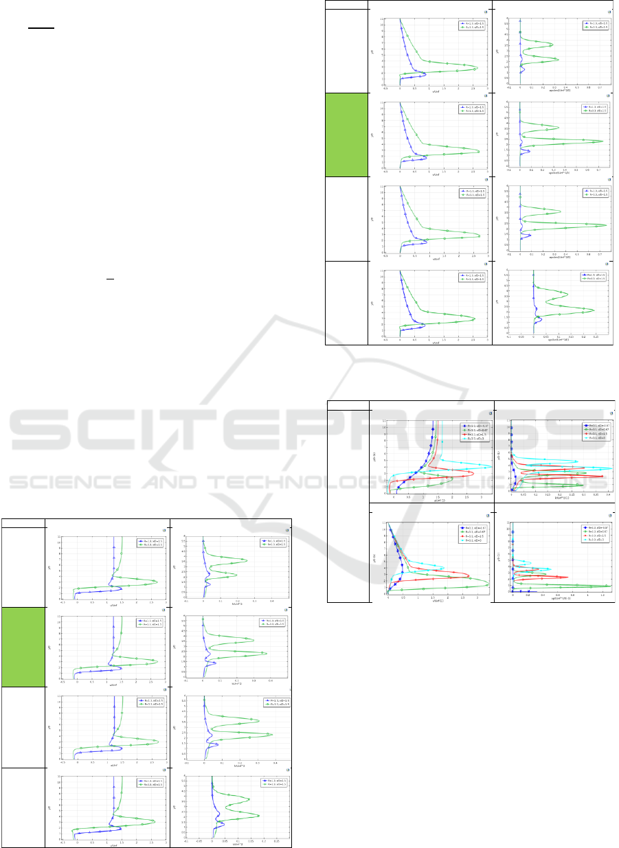
elements for modelling. The results for dimensionless
turbulent quantities; average velocity components
(
,
), kinetic energy (
), and energy
dissipation (
) are presented. These values are
computed for two cases; and . For each
case the variations of each quantity are presented at
several locations along the main stream channel.
These locations (
are
selected such that the model results could be
compared with those from the references for
validation, see Table 3.
The results agree, with acceptable accuracy, with
those of existing experimental and numerical data,
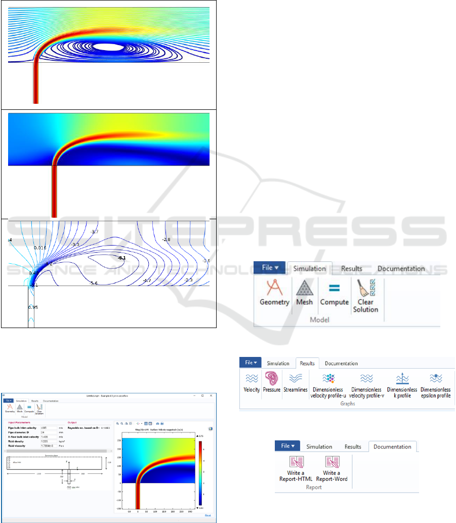
see Figures 4-6 in (Rodi, 2005). In addition, the
model produces maps of streamlines, velocity
magnitude, and pressure contours as shown in Table
4, for . As shown, the recirculating zone
located at downstream of the jet is captured with good
accuracy. The length and depth of the recirculating
zone is of interest for industrial and environmental
Table 2: Results used for mesh sensitivity analysis.
Table 3: Model results for dimensionless turbulent
quantities.
applications. If required, the model results can be
used for generating the dimensions and
characteristics of the velocity filed map, pressure
contours, and recirculating zone streamlines with
higher resolution.
5 MODELLING APP
For practical applications, it is preferred having a tool
besides CFD model which can be used by designers
and engineers. For this purpose, we built an App
using COMSOL tools. This App is based on the
model developed and can run independent of the
model. The latest version of the software (i.e., version
Mesh
u/U
∞
k/ U
2
∞
Structured-
Mesh1:
Number of
elements
33280
Structured-
Mesh2:
Number of
elements
133120
Structured-
Mesh3:
Number of
elements
299520
Unstructured:
Number of
elements
20217
Mesh
v/U
∞
/ U
3
∞
Structured-
Mesh1:
Number of
elements
33280
Structured-
Mesh2:
Number of
elements
133120
Structured-
Mesh3:
Number of
elements
299520
Unstructured:
Number of
elements
20217
Mesh
u/U
∞
profiles
k/ U
2
∞
profiles
Structured-
Mesh2:
Number of
elements,
133120
v/U
∞
profiles
/ U
3
∞
profiles
Turbulent Flow Modelling of a Jet in a Cross-Flow Stream: Model and App
199
5.4) enables users building a license-independent App
as *.exe type file using a COMSOL model. Hence,
one doesn’t require the software license for App
execution.
Table 4: Model results; streamlines, velocity magnitude,
and pressure contours maps close to the jet inflow.
The App presented here provides users modelling
facilities to study and model a jet flow entering a main
cross stream manipulating input data. A screen
capture of the App’s interface is shown in Figure 2.
Figure 2: App user interface.
As shown, the interface has three tabs; Simulation,
Results, and Documentation. The data can be entered
under the Input Parameters section. The resulted
Reynolds number appears in the Output section.
The Graphics window shows Geometry, Mesh,
and a series of modelling results, when desired. A
sketch of the modelling domain geometry is shown in
the interface in order to help users for identifying
input data and parameters. By clicking on the
Simulation Tab, four buttons appear in the ribbon bar,
as shown in Figure 3. By clicking on the Geometry
button, the latest geometry of the model appears in the
Graphics window. Similarly, the Mesh button would
show the structured mesh build in the flow domain.
The Compute button, when clicked on, would run the
model. A green progressive bar appears on the bottom
right-hand corner of the Interface window, indicating
the calculations. Once the calculation is complete a
default velocity plot appears in the Graphics window.
By clicking on the Results Tab, seven buttons
appear in the ribbon bar, as shown in Figure 4. The
label for each button describes the type of results
plotted in the Graphics window, when that button is
clicked on. By clicking on the Documentation Tab,
two buttons appear in the ribbon bar, as shown in
Figure 5. By clicking on these buttons, a report is
generated. Two formats are provided; HTML and
Word™. The App provides the option for saving the
generated Report with the desired file name.
Figure 3: App Simulation Tab.
Figure 4: App Results Tab.
Figure 5: App Documentation Tab.
SIMULTECH 2019 - 9th International Conference on Simulation and Modeling Methodologies, Technologies and Applications
200

6 CONCLUSION
A model and an App are built for analysing and
designing the turbulent flow of a jet entering a cross-
flow main stream, using COMSOL. The model
results are compatible within acceptable accuracy
with the cited references existing results, considering
that the model is built in a 2D domain and the existing
experimental results are in 3D. The App is built to
help with related practical applications of the model
and facilitates parametric analysis of the flow
behaviour.
REFERENCES
Ozcan,O. and Larsen,P.S, Report MEK-FM 2001-02. An
Experimental study of a turbulent jet in cross-flow by
using LDA, s.l.: Technical University of Denmark.
Rodi, W. (., 2005. Comparison of Turbulence Models in
Case of Jet in Crossflow using Commercial CFD Code.
In: Engineering Turbulence Modelling and
Experiments 6: ERCOFTAC International Symposium
on Engineering Turbulence and Measurements -
ETMM6. s.l.:Elsevier, pp. 399-408.
Tabatabaian, M., 2015. CFD Module: Turbulent Flow
Modeling and Turbulent Jet stream in a cross flow
COMSOL model and App.. s.l.:Mercury Learning and
Information.
Turbulent Flow Modelling of a Jet in a Cross-Flow Stream: Model and App
201
