Accelerating Urban Modelling Algorithms with Artiﬁcial Intelligence

Richard Milton

and Flora Roumpani

Centre for Advanced Spatial Analysis, University College London, 90 Tottenham Court Road, WC1E 6BT, U.K.

The Alan Turing Institute, The British Library, London, U.K.

Keywords:

Urban Modelling, Spatial Interaction Modelling, Artiﬁcial Intelligence, 3D Visualisation.

Abstract:

In this paper, we demonstrate that developments in computer hardware to support the increasingly complex

artiﬁcial intelligence workﬂows for Deep Learning networks can be adapted for urban modelling and visual-

isation. The hypothesis here is that by leveraging the current practice of AI as a Service (AIaaS), then this

enables Urban Modelling as a Service (UMaaS) to be developed. The starting point for this paper is a 3D vi-

sualisation of the Queen Elizabeth Olympic Park, developed using a web-based spatial interaction modelling

system which calculates population metrics on the ﬂy, capable of showing the results of interventions by urban

planners in real-time. We take the web application that powers the interactive visualisation and use Google’s

TensorFlow AI library to accelerate the matrix operations required to run the spatial interaction model, making

the web application fast enough to be used interactively.

1 INTRODUCTION

This work takes our existing ‘QUANT’ website for

spatial interaction modelling (ﬁgure 1) and uses its

core modelling services in an interactive 3D planning

scenario based around housing requirements for the

Queen Elizabeth Olympic Park. Our stated aim is to

use AI hardware acceleration to build an ‘urban mod-

elling as a service’ system to provide urban planners

with the ability to build their own applications, exper-

iment and see immediate results. This then allows us

to take a step further, and we test a number of neural

spatial interaction models, asking the question about

which mathematical model best ﬁts the data.

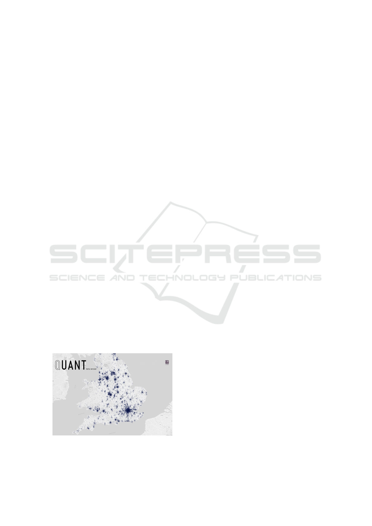
Figure 1: The QUANT Website, http://quant.casa.ucl.ac.uk,

showing the travel to work ﬂows.

While the links between artiﬁcial neural net-

works (ANNs) and spatial interaction models have

been cited in the literature as far back as (Fischer

and Sucharita, 1994), (Black, 1995) and (Openshaw,

1997), recent advances in specialised computing ar-

chitectures designed to accelerate the matrix opera-

tions required to train a large-scale deep neural net

have now become mainstream. As a consequence of

this, open-source libraries such as TensorFlow (Abadi

et al., 2016), Keras (Chollet, 2015), PyTorch (Paszke

et al., 2017) and Caffe (Jia et al., 2014), can rou-

tinely deal with ANNs that are orders of magnitudes

larger than a previous generation. These libraries are

designed to work on conventional CPUs for small-

scale work, in addition to utilising the multiple par-

allel cores of graphics processing units (GPUs) for

large-scale networks. Add to this the Tensor Process-

ing Units (TPUs), designed by Google for AI work-

ﬂows at the level of warehouse scale computing, plus

a myriad of other custom hardware for vision and

speech processing ‘at the edge’ (e.g. MOVIDIUS

Neural Compute Stick (Intel, 2019)) and the poten-

tial exists to make use of this high performance cloud

and desktop processing capability. The natural ques-

tion to ask is how to make a symbiotic link between

the current advances in AI and existing urban mod-

els? This paper sets out to put urban modelling into

the context of mainstream AI to both accelerate the

current computer models and to suggest new avenues

Milton, R. and Roumpani, F.

Accelerating Urban Modelling Algorithms with Artiﬁcial Intelligence.

DOI: 10.5220/0007727201050116

In Proceedings of the 5th International Conference on Geographical Information Systems Theory, Applications and Management (GISTAM 2019), pages 105-116

ISBN: 978-989-758-371-1

105

for future research. Existing applications of “AI as

a Service” can be cited which relate to object and

speech recognition, natural language processing and

other artiﬁcially intelligent systems, but there is an

absence of applications relating to urban modelling.

While one discipline seeks to give computers human

abilities, the other seeks to explain and predict hu-

man behaviour. A commonality exists where the pat-

tern matching abilities of ANNs are compared and

contrasted with the calibration and ‘model parameter

ﬁtting’ phase common in many types of urban mod-

elling. In effect, both are seeking to minimise an error

term and ﬁnd the best ﬁt for the data available.

The decision to focus on spatial interaction mod-

elling is based on the already established theoretical

links with ANNs, which are expanded upon in section

2. The initial work on QUANT developed a website

for spatial interaction modelling using 7,201 zones

for England and Wales. This is introduced in sec-

tion 3 and provides the real-life urban planning sce-

narios used to test the algorithmic and architectural

improvements. The urban datasets used in QUANT,

for example the travel times between zones and trip

matrices, are re-used in this paper, which extends the

urban modelling system beyond the current capabili-

ties of the QUANT system. This is a step-change in

performance, as, while QUANT takes around 10 sec-

onds to run a model, the system presented here takes

just 0.28 seconds. The modular and web-based design

of the system means that these improvements can be

easily incorporated and used with both 2D and 3D vi-

sualisation workﬂows. As an application of the the-

ory, we present the Queen Elizabeth Olympic Park

(QEOP) urban planning example, which is a Unity

application that requires the immediate urban mod-

elling enabled by the work in this paper. Unity is a

3D game engine development environment, which is

introduced in, “Unity 3D Game Development by Ex-

ample” (Creighton, 2010). While this serves as a vi-

sual front-end for planners who use the system, by

improving the performance of the spatial interaction

modelling algorithms, we demonstrate a step in per-

formance that makes the immediate urban modelling

required by the 3D application possible.

2 RELATED WORK

In his 1997 book, “Artiﬁcial Intelligence in Geogra-

phy” (Openshaw, 1997), Openshaw demonstrates the

application of an ANN to a spatial interaction mod-

elling problem involving ﬂows of people. Following

on from this, in “Building an Automated Modeling

System to Explore a Universe of Spatial Interaction

Models” (Openshaw, 1998a), a ‘universe’ of mod-

elling equations is ﬁtted to calibration data in an at-

tempt to ﬁnd the equation that describes the data with

the lowest error. The interesting result here is that

the traditional gravity model equations do not give the

best ﬁt with the training set. In all of these examples,

the inputs to the models are the origin and destination

attractions, derived from the ﬂows, and the distance

between zones. For the purposes of the following

discussion, a singly constrained spatial interaction, or

gravity model, is deﬁned by the following equation:

i j

= A

−βc

i j

(1)

∑

−βc

i j

(2)

i, j = origin and destination zone numbers,

i j

= cost of travel between them,

β = parameter for willingness to travel given cost,

= origin attraction,

= destination attraction,

= balancing factor

An important distinction to make concerns the

number of degrees of freedom of the model and the

method of training or calibration. In a spatial inter-

action model, the calibration involves ﬁtting a pa-

rameter, β, that deﬁnes how far people are willing

to travel. In Openshaw’s neural spatial interaction

model, the net has been trained to predict ﬂow from

origin (O

) and destination (D

) attractions at the in-

put layer. The β parameter is learnt by the network

as a ‘black box’, which could explain why neural spa-

tial interaction modelling techniques are not widely

adopted. However, the point being made here is one

of equivalence and some of the beliefs of neural nets

as being black boxes that defy explanation are chal-

lenged in the remainder of this paper. Here we argue

that black boxes are not the only option, advocating a

different approach which leads to “Urban Modelling

as a Service” for the exploration and explanation of

different scenarios. By way of comparison with equa-

tion 1, a simple ‘feed forward’ neural network is de-

ﬁned as follows:

∑

k j

(3)

= ϕ(v

) + θ

(4)

= neuron k internal state,

k j

= weight between input j and neuron k,

= input to neuron j,

= neuron output,

ϕ = activation function,

= bias value

GISTAM 2019 - 5th International Conference on Geographical Information Systems Theory, Applications and Management

106

In “Spatial Interaction Models: From the Gravity

to the Neural Network Approach” (Fischer and Reg-

giani, 2005), Fischer and Reggiani discuss different

forms of spatial interaction models, from singly and

doubly constrained through to a singly constrained

neural spatial interaction model, including the choice

of activation function (ϕ(v

) in equation 3). Their

conclusion states that the classic gravity model equa-

tions (equation 1) are the preferred choice because

of the “simplicity of their mathematical form and the

theoretical nature of their underlying assumptions”.

However, they go on to say that the neural network

approach is attractive in “data-rich environments” and

where “little is known about the form of the spatial

interaction function to be approximated”. In “Why

does deep and cheap learning work so well?” (Lin

et al., 2017), Lin shows how a three layer continu-

ous input feed forward network can be made to ap-

proximate a gate multiplier to any degree of accuracy.

Their analysis of the types of functions that deep neu-

ral networks can be made to approximate is impor-

tant in the context of modelling when the function

underlying the observed data is under investigation.

This ﬁnal point ﬁts with our statement in the intro-

duction about discovering new avenues of research.

The initial research with our previous QUANT model

was to see whether a large-scale model covering the

whole of England and Wales was possible. One of the

difﬁculties with spatial interaction modelling is that

the algorithm is of order O(n

), while the number of

zones, n, can be in the thousands in order to combat

edge effects and demonstrate the ﬁner grain detail of

the model. It should be noted that the QUANT sys-

tem currently runs equation 1 in 1.23 seconds on an

8 core CPU using parallel optimisations

, while a test

using OpenCL achieved the same result, but taking

only 0.25 seconds. This test was using dual NVIDIA

GTX 980 Ti GPUs, each with 640 cores clocked and a

quoted speed of 1306 GFLOPS. This evidence forms

our basis for believing that urban modelling can be

inﬂuenced by the current pace of AI research. One

thing stands out about equation 1 above all else. It is

‘pure parallel’, in that there are no loop dependencies

between different i or j indexes, so every T

i j

can be

calculated independently without having to wait for

a prior dependency. This fact, which is backed by

the evidence in the following results section, is the

cornerstone of our argument. The re-formulation of

the spatial interaction model equations into a parallel

form enables maximum usage of all available process-

ing cores on any massively parallel architecture.

The gravity model formula in equation1 needs to exe-

cute n x n times to compute every value in the matrix where

n = 7201 zones, giving rise to ≈ 52million iterations.

The ﬁnal point to note regards the number of zones

in the model. While Black’s example (Black, 1995)

had 9 zones, Openshaw’s example of Durham had

73 zones. The example here has 7,201 zones for the

whole of England and Wales, so the goodness of ﬁt of

a neural spatial interaction model of this size is one

metric to be investigated, as it is possible that the net-

work might not train on a model of this size. Also, the

observed matrix contains 51, 854, 401 training sam-

ples.

In the following sections we demonstrate our cur-

rent work on building a web-based urban modelling

framework. The key consideration inﬂuencing the de-

sign is for immediate results, rather than having to

wait hours for a simulation to run, as was the case in

the past. This focuses our work on urban modelling

for experimentation and exploration.

3 OVERVIEW

Previously, it has not been possible to create models

with the number of zones we require and that also run

fast enough on the hardware to make “Urban Mod-

elling as a Service” (UMaaS) a viable proposition.

Our method enables this through a set of web ser-

vices acting as a “model view controller” and provid-

ing the client with a REST API for the urban mod-

elling functions. As this is a real-time modelling ser-

vice, the main requirement is to provide the user with

model outputs fast enough to be interactive. In or-

der to achieve this, we use the software and hardware

improvements being driven by “AI as a Service” to

power “Urban Modelling as a Service”.

While equation 1 introduced the basic gravity

model equation, there are four variants that are de-

ﬁned as follows: unconstrained, singly constrained

origin, singly constrained destination and doubly con-

strained. A complete description can be found in

“A Family of Spatial Interaction Models” (Wilson,

1971). For simplicity, the results presented here fo-

cus on the singly constrained origin model, but the

results are directly applicable to all four variants.

Of paramount importance to our case for ‘urban

modelling as a service’ is the quantity and variety of

data required to build a real urban model, as opposed

to a theoretical example. The data required for the

model are: zone boundaries, zone centroids, network

graphs for each mode of travel (e.g. road, rail, bus),

cost function between zones per mode of travel (c

i j

resident population, workplace population, travel to

work ﬂow matrix per mode (T

i j

), land use (building

constraints on space), green belt, parks and protected

areas.

Accelerating Urban Modelling Algorithms with Artiﬁcial Intelligence

107

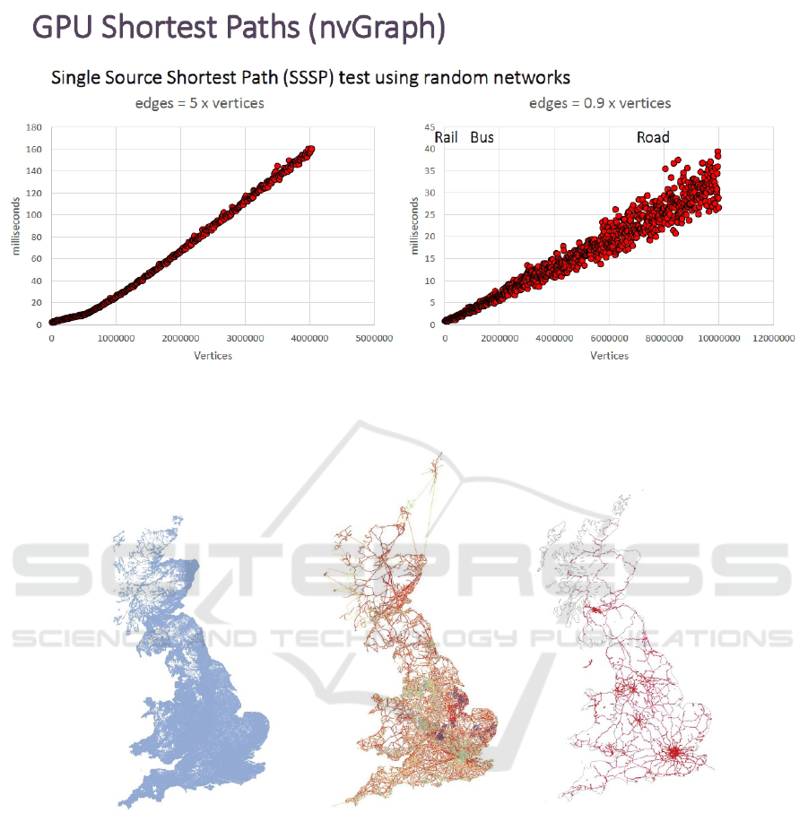
Figure 2: Single Source Shortest Path runs on random networks with varying numbers of vertices. The graph on the right is

for a sparse network (e = 0.9v), while the left graph is more highly connected (e = 5v). The relative positions of the rail, bus

and road networks are shown on the graph to give a sense of scale.

Figure 3: Left: road network (8.4M edges), Centre: bus network (0.42M edges) and Right: rail network (10,269 edges).

The cost function is required for every zone pair

and mode, yielding an n x n matrix that matches the

dimensions of the ﬂow matrix. This is signiﬁcant

undertaking computationally when n = 7201 =⇒

51, 854, 401 trips, where each trip requires running

a shortest path algorithm to obtain the minimum trip

time on a network graph containing 8 million edges.

Figure 3 shows the three transport networks behind

how the cost matrices are calculated. The two graphs

in ﬁgure 2 show the application of Nvidia’s nvGraph

library to this problem. While the cost matrices used

in this paper use the real transport network for Eng-

land and Wales (ﬁgure 3), the tests in ﬁgure 2 are for

randomised networks with two variations on the ratio

of the number of edges to the number of vertices.

4 APPLICATION

The current release of QUANT, simulates the im-

pact of changes in population, employment and travel

costs in UK Cities, using a simple model of how

workers choose where to live in respect to the attrac-

tiveness of those places and the cost of traveling to

their workplaces. By building this as a set of web ser-

vices, the core modelling component can be re-used

GISTAM 2019 - 5th International Conference on Geographical Information Systems Theory, Applications and Management

108

Figure 4: The Unity 3D Olympic Park application. A scenario built using the QUANT web services core (ﬁgure 5).

in other scenarios. The following sections describe

how the QUANT urban modelling services are used

in a 3D interactive planning application for the Queen

Elizabeth Olympic Park (ﬁgure 4). The application

tests scenarios online by assigning proposed increase

in employment, and by calculating ﬂows of popula-

tion based on a singly constrained spatial interaction

model. These are based on three means of transporta-

tion: tube, buses and trains. As such it can calculate

inter-city ﬂows that come from not only within Lon-

don, but from all of the UK.

This is very useful for the evaluation of master-

plans for areas in metropolitan cities such as Lon-

don. For example, The London Legacy Development

Corporation (LLDC) is now using the opportunity of

the London 2012 Games and the opening of Queen

Elizabeth Olympic Park (QEOP) to create “a dynamic

new metropolitan centre for London, and develop an

inspiring and innovative place where people want –

and can afford – to live, work and visit” (LLDC,

2011). The plans include large scale residential de-

velopments and supralocal commercial centres such

as Westﬁeld London, that are programmed to attract

people from all over London and beyond. As such

it cannot be studied in isolation, and would be useful

to include a regional model that calculates ﬂows of

employment and population in order to program the

capacities needed for transportation, housing and ser-

vices.

We will use QUANT MSOA zones as the regional

zones (I,J), whose modelling outputs can be accessed

real time using requests from the web server using

QUANT’s REST API, and develop a ﬁne scale plan-

ning zone system for the Olympic Park in the Unity

3D graphics package. Essentially, we develop a sys-

tem, in which we design new developments, these will

be translated into ﬂoorspace, and then to population.

This means, that it is possible to create scenarios by

calculating the total of employment and population

from all planning zones within each MSOA in the

Olympic Park and then send it back to QUANT to

calculate ﬂows on a regional level. This loop will en-

sure the stability of the planning scenarios, and allow

QUANT and the planning model to communicate by

exchanging information back and forth.

To create the ﬁne-scale planning zones we use

the ofﬁcial planning policies of the QEOP as set by

LLDC. These indicators will essentially inform the

design scenarios with permissions set by the different

urban authorities. We can then develop a calibrated

urban planning model as an internal pre-model which

will take the role of assigning population ﬂows from

Accelerating Urban Modelling Algorithms with Artiﬁcial Intelligence

109

the QUANT regional model to the designed planning

zones. This follows the initial work visualising com-

plex urban models in procedural 3D environments

(Roumpani et al., 2013) ,(Hudson-Smith, 2014). In

this case we have linked building ﬂoorspace and land

uses with population ﬁgures. e.g. A housing unit of

300m

hosts maximum 10 people. The result of this

work, is then a composite interactive 3D plan of the

Olympic Park, which links ﬂoorspace as designed in

Unity3D with population projections from QUANT.

Starting with the existing conditions of the Park and

adding the projected developments of the LCS, we

set out to show how the assigned development types

would affect growth over the projected period, and to

compare alternative development strategies. We have

developed this as an android application, which uses

the 3D model as an interface (ﬁgure 4). This will al-

low the user to experiment with different policies and

test scenarios within a 3D model of the Olympic park

and use QUANT to evaluate these scenarios in terms

of population distribution.

5 IMPLEMENTATION

In this section we present our architecture for running

urban modelling experiments, followed by an analysis

of the achieved performance in the ‘Results’ section.

At the top level, this consists of a collection of web

services using a ‘model view controller’ pattern. The

structure of this can be seen in ﬁgure 5. Below the

web services layer are the libraries that perform the

actual modelling functions. This enables us to sep-

arate the functionality from the web protocol frame-

work and test the performance of the urban modelling

library in isolation. By exposing the modelling func-

tions as a set of web services, different clients can be

used for exploration and visualisation. In the process

of our testing we used both conventional 2D maps and

a 3D client written using the Unity framework. For

the purposes of this paper, though, only the “QUANT

Model” and “Web Services” boxes are considered as

these deal with the calibration and the running of the

model.

The rest of this section describes the implementa-

tion of the modelling library as follows:

1. CPU based spatial interaction model

2. GPU based spatial interaction model (OpenCL)

3. AI optimised spatial interaction model (Tensor-

Flow)

4. AI optimised neural spatial interaction model

(Keras/Tensorﬂow)

5. AI alternative model structure (radial basis, gener-

ative adversarial networks, neurodynamic models

(Milton et al., 2018))

This methodology allows 1, 2 and 3 to be com-

pared for speed as they are functionally identical,

while 4 and 5 are interesting from a research point

of view as they explore modelling equations them-

selves. The implementation is using Python 3.6 as

it allows for a TensorFlow implementation with the

trained model able to be run on the CPU or GPU for

benchmarking.

We start with an origin constrained spatial inter-

action model of commuter ﬂow in England and Wales

using data from the 2011 Census. Data is available at

the ‘Middle level Super Output Area (MSOA)’ geog-

raphy, where there are 7201 zones in the model.

i j

= O

−βc

i j

∑

−βc

i j

(5)

i<n

∑

i=0

i j

, D

j<n

∑

j=0

i j

(6)

The variables in equation 5 follow the same pat-

tern as equation 1, earlier, with the exception of B

which is a constraints factor, used to prevent build-

ing in zones where none is possible, for example on

green belt land, parks, or areas of outstanding natural

beauty. In terms of the system diagram in ﬁgure 5,

this ﬁts into the box labelled “QUANT Model”.

While commuter ﬂows have been used as the ini-

tial example (travel to work), other types of ﬂow are

also considered such as retail (travel to shop). As

long as there is some type of ﬂow matrix, T

i j

, then

anything can be simulated. In addition to this, ﬂows

can be disaggregated by type, so, in the case of travel

to work, the ﬂows are broken down into three modes

‘road (mode=0)’, ‘bus and tube (mode=1)’ and ‘heavy

rail (mode=2)’. This results in one order n x n matrix

i j

and one trip cost matrix c

i j

for each of the three

transport modes. The ﬁnal result is then given by the

following equation:

total

i j

m<3

∑

m=0

i j

, {m = mode} (7)

Learning in this respect is seen as ﬁtting the β pa-

rameter to achieve the optimal goodness of ﬁt mea-

sured over D

for singly constrained, or both O

and

for doubly constrained. The β parameter repre-

sents the willingness of a commuter to travel the dis-

tance between i and j, which is where the functional

difference between the conventional spatial interac-

tion model and the neural spatial interaction model

can be measured.

GISTAM 2019 - 5th International Conference on Geographical Information Systems Theory, Applications and Management

110

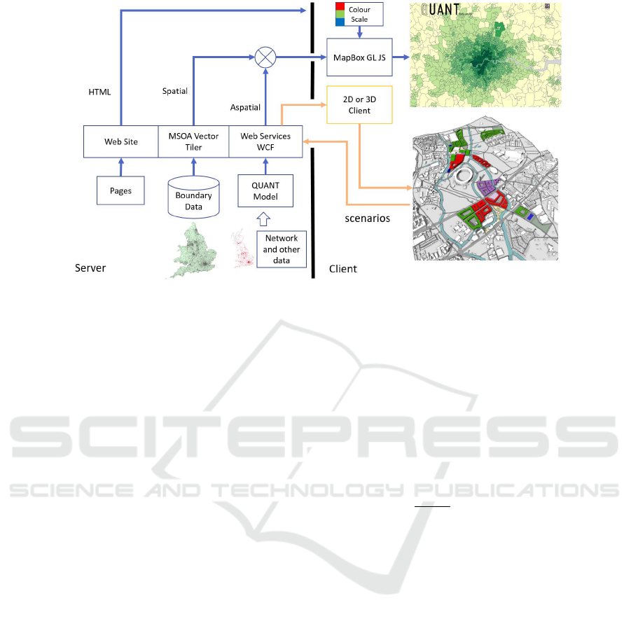
Figure 5: QUANT system diagram showing the server/client split. The box labelled “QUANT Model” contains the code

outlined in this paper. This is the section that is critical to the speed of the entire system.

For the TensorFlow version of the conventional

spatial interaction model, the operations required to

run the model are deﬁned by an execution graph. This

graph is shown in ﬁgure 6, which shows the paral-

lelism achievable in the ﬂows of dependencies. The

bar

calculation (mean trips) from T

i j

(trips matrix) is

visible, along with the O

and D

row and column sum

reductions. Other than the trips matrix, the only other

inputs to the system are C

i j

(cost matrix) and the β

parameter which is the variable to be calibrated. This

execution graph only shows a single run of the model

equation, with no adaptaion of the β parameter to ﬁt

the data to the observed values (T

i j

). The reason for

this is that this is the execution graph that was used for

the benchmark tests between the regular Python code

and the TensorFlow code to measure both speed of ex-

ecution and equivalence of numerical results. Adding

the β calibration to the graph is added in the produc-

tion version of the class, while the simpliﬁcation here

is to make direct testing possible.

All the code for this paper can be found

on GitHub under the following project:

https://github.com/maptube/UMaaS.

5.1 Neural Model

The neural spatial interaction model follows the pre-

vious work of Openshaw (Openshaw, 1997, pp174),

Black (Black, 1995) and (Fischer and Sucharita,

1994), using [O

, D

i j

] as inputs to the model with

i j

as the target. Openshaw included an additional ‘in-

trazonal ﬂag’, used to indicate when i = j and travel

is within the same zone. This has not been used here,

but one advantage of the neural model over the con-

ventional spatial interaction model is that additional

parameters can be added as inputs to explore their

signiﬁcance, as discussed in (Openshaw, 1998a). An-

other problem concerns the scaling of the inputs and

outputs, which need to be in the range [0..1] for the

neural network type used here. The practice adopted

in the literature is used, with the inputs and outputs

being scaled linearly. This introduces a problem, as

the maximum O

value is 24, 061, resulting in a scal-

ing factor of

max(O

)

= 4.15x10

−5

. This needs to

be applied to the loss function, used to establish the

model’s goodness of ﬁt when training.

Having deﬁned the inputs and outputs, the next

problem concerns the network structure itself. While

three inputs and one output is ﬁxed, the number of

hidden layers in between can be varied, as can the

number of neurons in each layer. This introduces an

optimisation problem where too few layers and neu-

rons results in the model not ﬁtting the observed data

to a high enough level of accuracy, while too many

will result in over-ﬁtting the model. Black (Black,

1995) used a single hidden layer, obtaining results

better than the conventional formulation of the model,

which suggests that one layer is adequate. Fischer

(Fischer and Sucharita, 1994) evaluated ten different

network architectures, varying the number of hidden

neurons in order to ﬁnd the optimum for his telecom-

munications data. Our zonal model is an order of

magnitude bigger than any in the literature (Black 9

zones, Openshaw 73 zones), so the structure of the

network is under investigation. Finally, the activation

function, ϕ() in equation 3, needs to be chosen. In

Accelerating Urban Modelling Algorithms with Artiﬁcial Intelligence

111

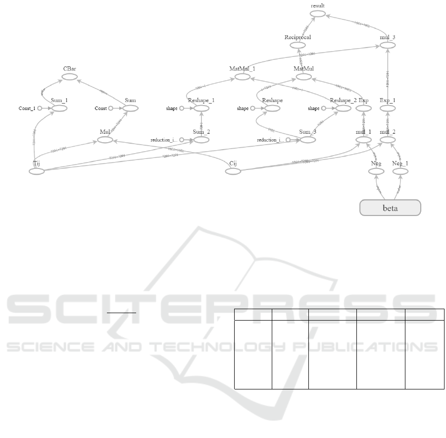
Figure 6: Tensorﬂow execution graph for the TFSingleOrigin code to run the conventional model of equation 5 on the GPU.

“Spatial Interaction Models: From the Gravity to the

Neural Network Approach” (Fischer and Reggiani,

2005), Fischer and Reggiani use the sigmoid, or lo-

gistic function, deﬁned as follows:

ϕ(x) =

1 + e

−x

(8)

The ANN model is implemented using the Keras

library. While this could be implemented directly us-

ing TensorFlow, the advantage of using a higher level

library over the lower level TensorFlow library is the

ease with which different neural network architec-

tures can be explored. In the older literature cited

at the beginning of this section, three layer networks

with a single hidden layer were used. Here, we inves-

tigate the effect of adding additional hidden layers on

the prediction performance using a parameter sweep

of number of layers and number of neurons. During

training the error is taken as mean square error be-

tween output and target summed over the batch. A

single epoch represents all of the trips data available

being applied in batches.

The following data is an example from the training

set, which contains 1,960,428 non-zero patterns from

original census data, or 3.78% of the full 7201x7201

matrix.

[ Oi, Dj, Cij ] ---> Tij

[ 24061.0 , 165.0 , 1.0 ] ---> 19.0

[ 24061.0 , 1006.0 , 13.0 ] ---> 8.0

[ 24061.0 , 1645.0 , 11.0 ] ---> 11.0

[ 24061.0 , 1248.0 , 13.0 ] ---> 13.0

[ 24061.0 , 1419.0 , 11.0 ] ---> 18.0

[ 24061.0 , 1241.0 , 12.0 ] ---> 9.0

For the purposes of evaluating the performance of

the neural model, six different network architectures

were tested, as shown in table 1.

Table 1: Network architecture.

Model Inputs Hidden 1 Hidden 2 Output

1 3 64 0 1

2 3 32 0 1

3 3 16 0 1

4 3 8 0 1

5 3 4 0 1

6 3 4 4 1

The network architectures were chosen as follows:

model 1 is larger than Openshaw’s test in (Openshaw,

1998b), which had a maximum of 50 hidden neurons,

while model 5 is smaller than his minimum of 7. This

is included as a test to allow a fast executing model to

be trained for longer. Finally, model 6 is a deep net-

work, included as a comparison with the single hidden

layer architectures. While the conventional spatial in-

teraction model can be approximated to any degree

using a single hidden layer, the deep network is to test

whether a more complex function can be discovered

which ﬁts the data more closely.

Benchmark tests were run on a cropped version of

the England and Wales data, consisting of a 500 zone

segment of London. This was necessary to reduce

the training time and allow a parameter sweep of the

number of hidden neurons, number of layers, batch

size and number of training epochs. With the full

England and Wales, data, there are 51, 854, 401 in-

GISTAM 2019 - 5th International Conference on Geographical Information Systems Theory, Applications and Management

112

put/target training pairs compared to 250, 000 for the

smaller subset of London, so this represents a signiﬁ-

cant reduction in compute time. Training is based on

minimisation of “mean square error” over the batch,

with a batch size of 200, 000 to ﬁt inside GPU mem-

ory. Batches are presented for training in a random

order, which is a technique designed to prevent over-

ﬁtting the data.

Following the parameter sweep with the test

model, experiments were then conducted using the

full 7201 zone model for direct comparison with the

conventional gravity model.

6 RESULTS

This section presents the results of testing the ﬁ-

nal evolution of the code optimisations. The com-

puter used to do the tests is an Alienware Area 51

computer, i7 5960X @ 3GHz, 32GB RAM, dual

NVIDIA GTX980 Ti GPUs. For the Google Tensor-

Flow tests, this used TensorFlow version 1.12 with

NVIDIA CUDA Toolkit 9.0. For the purposes of test-

ing, ﬁgure 7 shows the results of executing the main

spatial interaction model given by equation 5. This is

the base equation used in both the calibration (train-

ing) phase and later for inference, or testing scenarios.

Where a multi-modal model is concerned, each mode

is computed separately using the same equation, so

this serves as a representative test.

The TensorFlow model class

is used to build the

graphs for the O

and D

inputs to the model equa-

tion, which are row and column sums computed using

a reduction kernel. One of the problems with measur-

ing GPU performance is that there is signiﬁcant setup

time compared to the CPU, the effects of which have

been minimised by timing batches of 1000 runs of the

code.

For comparison, a C# implementation was con-

structed to match the Python implementation. This

runs the benchmark test on a matrix of size 7201 in

1.23 seconds, compared to the Python implementa-

tion presented here, which takes 1.54 seconds on the

same test.

6.1 Neural Model Results

While Tensorﬂow and GPU hardware has been used

to accelerate the evaluation of the conventional grav-

ity model, this section presents the results of training

an artiﬁcial neural network (ANN) on identical trips

TFSingleOrigin: https://github.com/maptube/UMaaS/

blob/master/models/TFSingleOrigin.py

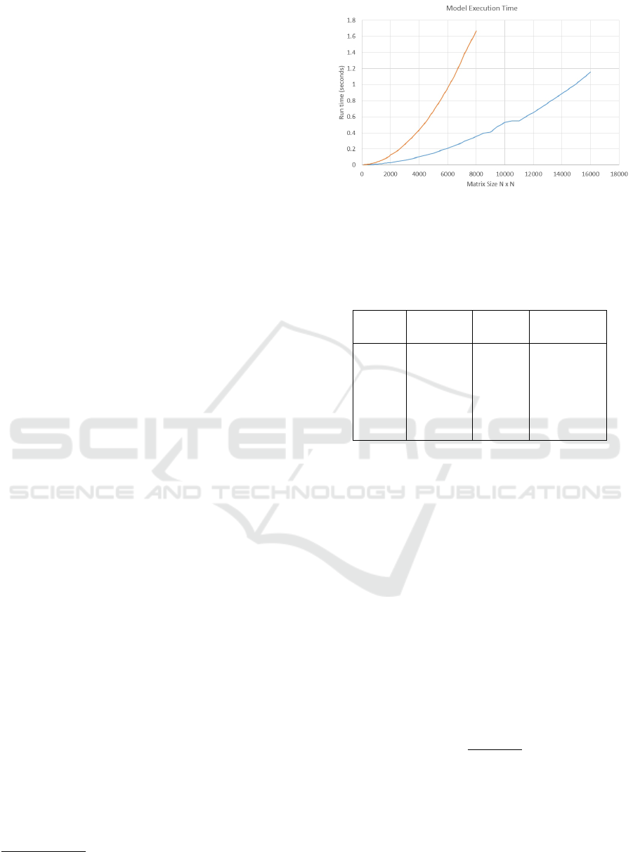
Figure 7: Model execution time graph showing the effect

that changing the matrix size has on the model run time.

Timings are in seconds for a single model run, based on an

average of 1000 runs on the CPU or GPU.

Table 2: Training time for 10,000 epochs and ﬁnal error.

NOTE: this is for the 500 x 500 test matrix.

Model Net Training

Time

Min Error

(

1 3-64-0-1 55min 0.65

2 3-32-0-1 33min 0.80

3 3-16-0-1 23min 0.18

4 3-8-0-1 19min 0.017

5 3-4-0-1 17min 0.19

6 3-4-4-1 19min 0.033

data. Firstly, the ANN has more degrees of freedom

than the β parameter of the gravity model. Here, the

model has three inputs, one or more hidden layers and

an output layer containing a single neuron. For a hid-

den layer with h hidden neurons, there are 3h weights

in the hidden layer and h weights in the output layer.

This makes calibration time longer than in the gravity

model case as shown in table 2.

In order to measure the goodness of ﬁt of the mod-

els, the

C metric is used, which is a measure of the to-

tal trip time recorded in the original observation data.

During the calibration phase of the conventional grav-

ity model, the β value is adjusted until the mean trip

times factor,

C is within 0.1 of the observed value.

Equation 9 deﬁnes how

C is calculated, with the val-

ues for each of the models shown in table 2.

C =

∑

i, j

i j

∑

i, j

i j

(9)

Training only needs to be performed once, though,

while speed of inference is the main metric of inter-

est. The test here is to see whether the mathematically

complicated ANN can be used to infer the data for the

entire N × N trips matrix in a time comparable to the

gravity model by using the hardware acceleration pro-

vided by the GPU.

Accelerating Urban Modelling Algorithms with Artiﬁcial Intelligence

113

Then, as a secondary test, the results are compared

with the conventional gravity model to see whether

they are consistent. Table 3 shows the inference times

for the full 7201 matrix data.

Table 3: Inference times for the full 7201 element matrix

data on the six models.

Inference Time (secs)

Model Net GPU CPU

1 3-64-1 1.156 74.937

2 3-32-1 1.025 14.523

3 3-16-1 1.214 5.314

4 3-8-1 0.900 3.240

5 3-4-1 0.929 2.152

6 3-4-4-1 0.996 3.590

Now, the goodness of ﬁt between the ANN model

and the observed data is measured. However, with

the neural model, training uses the mean square er-

ror between predicted and target as the loss function,

so the back-propagation algorithm seeks to minimise

this factor instead. This marks an important differ-

ence of the neural model, as the

C calculation requires

the entire predicted matrix for its evaluation, while the

neural model operates at the level of batches of indi-

vidual predicted/target pairs. This leads to the result

that the neural model’s mean square error is not di-

rectly comparable with

C, the usual measure of ﬁt for

a gravity model. The

C metric is trips weighted by

travel time, while the ANN’s loss algorithm only op-

timises for the raw number of trips. The mean square

error provides an upper bound on

C, which can be

seen in the data if

C is plotted against mean square

error.

Looking at the training data in ﬁgure 8, any of the

models with a ﬁnal error below 0.1 would be accept-

able in the context of the conventional gravity model,

which is calibrated to this accuracy. In other words,

we have a universe of models that provide a differ-

ent way of ﬁtting the observed ﬂow data. While ﬁg-

ure 8 shows the training on a test matrix of 500x500

for speed, this is still only a subset of the full data.

The faster training speed on this smaller data set en-

ables a parameter sweep which then translates into

faster training on the full 7201x7201 data set, which

is a factor of 207 times bigger. Although the smaller

matrix size was used as a test, it still constitutes real

data and could, in theory, be used to ‘seed’ the train-

ing with the full data. This has not been attempted

here, with the full training performed starting from

randomised weights. Using the graph in ﬁgure 8 and

timings obtained from running the software, the “3-

64-1” model was rejected on the grounds that train-

ing would need at least 10,000 epochs at 30 seconds

each (83 hours), similarly for “3-32-1” and “1-16-1”.

The “1-4-1” model was rejected for being too small to

generalise the data, leaving the “1-8-1” and “1-4-4-1”

(approx 0.5s per epoch) models. The “1-4-4-1” model

would make for an interesting comparison being a two

layer deep network, but, unfortunately, it proved too

difﬁcult to train, requiring over 40,000 epochs.

the remaining “1-8-1” model, after 12,000 epochs of

training the

C mean tips length is 23.8, when the ob-

served data is 12.5, this is with a mean square error of

4.16x10

−6

. The main lesson learned from the train-

ing exercise is to train with the full data and update

the weights at the end of the epoch, rather than using

small batches and updating more frequently.

7 CONCLUSIONS

In this paper we showed how the performance of a

gravity model is speeded up using the TensorFlow ar-

tiﬁcial intelligence library and GPU hardware. We

compared the CPU performance of the model with the

GPU accelerated model and showed how large mod-

els approaching 10,000 zones can be handled at in-

teractive speeds. We termed this, “Urban Modelling

as a Service”, leveraging “AI as a Service” for urban

modelling. The immediacy of the results is important

here due to the interactive nature of the visualisation

and exploration of modelling scenarios through a real-

time, web-based, user interface. The power of this ar-

chitecture is that it opens up the possibility of testing

modelling scenarios to the general public. Data like

the trips and cost matrices, zone boundaries, and con-

straints can be held and curated on the server, thereby

providing all the data required for modelling in one

place.

A secondary result is the comparison of a neural

spatial interaction model with a conventional model.

Here, the scaling of inputs to ﬁt the sigmoid activa-

tion function and extended training times on the data

are shown to be a problem. This is unfortunate, as

the logical extension to this work is to continue with

the comparison between the neural spatial interaction

models and the conventional model and show that

the neural network is not a “black box”. The same

methodological testing can be applied to both types

of model in order to assess their function. The future

direction of this research is to investigate the ensem-

ble of models provided by this method when applied

to the same scenario.

The estimates of how long training would take are

based on analysing the drop in error over time.

GISTAM 2019 - 5th International Conference on Geographical Information Systems Theory, Applications and Management

114

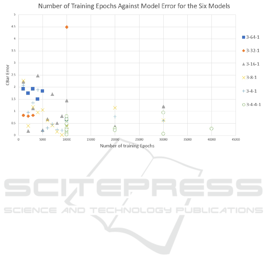
Figure 8: Number of training epochs and goodness of ﬁt (

C), this is for 500 x 500 matrix test data.

ACKNOWLEDGEMENTS

The authors would like to thank Prof. Andrew

Hudson-Smith for supervising the Queen Elizabeth

Olympic Park Unity 3D, Prof. Mike Batty for the

QUANT project and Prof. Alan Wilson (Alan Turing

Institute). We would like to thank EPSRC for fund-

ing the QEOP work under PhD grant number EPSRC

DTG 2012-2016.

REFERENCES

Abadi, M., Barham, P., Chen, J., Chen, Z., Davis, A., Dean,

J., Devin, M., Ghemawat, S., Irving, G., Isard, M.,

Kudlur, M., Levenberg, J., Monga, R., Moore, S.,

Murray, D. G., Steiner, B., Tucker, P., Vasudevan, V.,

Warden, P., Wicke, M., Yu, Y., and Zheng, X. (2016).

Tensorﬂow: A system for large-scale machine learn-

ing. In 12th USENIX Symposium on Operating Sys-

tems Design and Implementation (OSDI 16), pages

265–283.

Batty, M. (1976). Urban Modelling: Algorithms, Calibra-

tions, Predictions. Cambridge University Press.

Black, W. R. (1995). Spatial interaction modeling using

artiﬁcial neural networks. Journal of Transport Geog-

raphy, 3(3):159 – 166.

Chollet, F. (2015). keras. https://github.com/fchollet/keras.

Creighton, R. H. (2010). Unity 3D Game Development by

Example Beginner’s Guide. Packt Publishing.

Fischer, M. M. and Reggiani, A. (2005). Spatial interac-

tion models: From the gravity to the neural network

approach. In Capello, R. and Nijkamp, P., editors, Ur-

ban Dynamics and Growth: Advances in Urban Eco-

nomics, Contributions to Economic Analysis, volume

266, chapter 11, pages 319–346. Elsevier.

Fischer, M. M. and Sucharita, G. (1994). Artiﬁcial neural

networks. a new approach to modelling interregional

telecommunication ﬂows. Journal of Regional Sci-

ence, 34(4):503–527.

Hudson-Smith, A. (2014). Tracking, tagging and scanning

the city. Architectural Design, 84(1):40–47.

Intel (2019). Intel movidius neural compute stick. url

= https://software.intel.com/en-us/movidius-ncs. Ac-

cessed: Jan 2019.

Jia, Y., Shelhamer, E., Donahue, J., Karayev, S., Long, J.,

Girshick, R., Guadarrama, S., and Darrell, T. (2014).

Caffe: Convolutional architecture for fast feature em-

bedding. In Proceedings of the 22Nd ACM Inter-

national Conference on Multimedia, MM ’14, pages

675–678, New York, NY, USA. ACM.

Lin, H. W., Tegmark, M., and Rolnick, D. (2017). Why

does deep and cheap learning work so well? Journal

of Statistical Physics, 168(6):1223–1247.

LLDC (2011). LLDC legacy communities scheme. url

= http://www.queenelizabetholympicpark.co.uk/our-

story/transforming-east-london/legacy-communities-

scheme. Accessed: March 12 2018.

Milton, R., Hay, D., Gray, S., Buyuklieva, B., and Hudson-

Smith, A. (2018). Smart IoT and Soft AI. IET Con-

ference Proceedings, pages 16 (6 pp.)–16 (6 pp.)(1).

Openshaw, S. (1997). Artiﬁcial Intelligence in Geography.

John Wiley and Sons.

Accelerating Urban Modelling Algorithms with Artiﬁcial Intelligence

115

Openshaw, S. (1998a). Building an automated modeling

system to explore a universe of spatial interaction

models. Geographical Analysis, 20(1):31–46.

Openshaw, S. (1998b). Neural network, genetic, and fuzzy

logic models of spatial interaction. Environment and

Planning A: Economy and Space, 30(10):1857–1872.

Paszke, A., Gross, S., Chintala, S., Chanan, G., Yang, E.,

DeVito, Z., Lin, Z., Desmaison, A., Antiga, L., and

Lerer, A. (2017). Automatic differentiation in pytorch.

In NIPS-W.

Roumpani, F., O’Brien, O., and Hudson-Smith, A. (2013).

Creating, visualizing and modelling the realtime city.

In Proceedings of Hybrid City II ‘Subtle rEvolutions’

Conference.

Wilson, A. G. (1971). A family of spatial interaction mod-

els, and associated developments. Environment and

Planning A: Economy and Space, 3(1):1–32.

GISTAM 2019 - 5th International Conference on Geographical Information Systems Theory, Applications and Management

116