Detecting Inﬂuencers in Very Large Social Networks of Games

Leonardo Mauro Pereira Moraes and Robson Leonardo Ferreira Cordeiro

Institute of Mathematics and Computer Sciences, University of S

ao Paulo,

Keywords:

Data Mining, Social Networks of Games, Player Modeling, Classiﬁcation, Feature Extraction, Data Streams.

Abstract:

Online games have become a popular form of entertainment, reaching millions of players. Among these play-

ers are the game inﬂuencers, that is, players with high inﬂuence in creating new trends by publishing online

content (e.g., videos, blogs, forums). Other players follow the inﬂuencers to appreciate their game contents.

In this sense, game companies invest in inﬂuencers to perform marketing for their products. However, how to

identify the game inﬂuencers among millions of players of an online game? This paper proposes a framework

to extract temporal aspects of the players’ actions, and then detect the game inﬂuencers by performing a clas-

siﬁcation analysis. Experiments with the well-known Super Mario Maker game, from Nintendo Inc., Kyoto,

Japan, show that our approach is able to detect game inﬂuencers of different nations with high accuracy.

1 INTRODUCTION

The digital game market is in constant ascendancy,

both in the production and in the consumption. This

industry moves billions of dollars per year (Lucas,

2009). According to Newzoo

, a specialist company

of game marketing, the estimated value for 2018 is

US$ 134.9 billion. Only in the ﬁrst quarter of 2018,

players produced more than 260 million hours of on-

line videos related to game contents on Twitch and

YouTube platforms.

Online games are dynamic environments, in

which the players interact with the game and with

other players all over the world (Yannakakis and To-

gelius, 2015). The interactions performed by each

player represent relationships of several types; they

can relate to other players (e.g., friend, sharing games)

or to the game itself (e.g., play, like) (Lee et al., 2012).

These relationships form a social network, i.e., in this

context a Social Network of Games.

For example, the well-known Super Mario Maker

game (SMM), from Nintendo Inc., Kyoto, Japan,

forms a very large social network. According to Nin-

tendo

, it has more than 3.5 million players, and 7.2

million courses (or maps) that were already played

Newzoo. “Insights”. https://newzoo.com/insights/ (ac-

cessed December 18, 2018).

NintendoAmerica. “If you played every level

in #SuperMarioMaker for 1 minute each, it would

take you nearly 14 years to play them all!”.

https://twitter.com/NintendoAmerica/status/732624228428750848/

more than 600 million times. In this game, a player

can play, give a star, break a record or comment on

online courses created by other players, besides cre-

ating his/her own courses to share with the world.

Inﬂuencer users in the digital ﬁeld exist since

the popularization of social media (Pei et al., 2018).

They produce digital contents (e.g., online videos)

that arouse the attention of other users with similar

tastes. Among them, there are the game inﬂuencers

that produce contents related to digital games (Gros

et al., 2018; Hilvert-Bruce et al., 2018). Players fol-

low the game inﬂuencers looking for entertainment

and credible information on the universe of the games

(Sj

oblom and Hamari, 2017; Gros et al., 2018).

Game inﬂuencers get recognition from the play-

ers who follow them. Consequently, game companies

invest in inﬂuencers to endorse and perform market-

ing for their products (Sj

oblom and Hamari, 2017).

Hence, an inﬂuencer has direct relevance in such phe-

nomena as viral marketing, innovation diffusion and

behavior adoption (Pei et al., 2018). To detect game

inﬂuencers is therefore almost mandatory when look-

ing for popular preferences, new trends, and the like

(Sj

oblom and Hamari, 2017; Hilvert-Bruce et al.,

2018).

This paper proposes a novel framework to de-

tect game inﬂuencers in Social Networks of Games.

Given the actions of millions of players in an online

game, how to detect the game inﬂuencers? It is obvi-

(accessed November 10, 2018).

Moraes, L. and Cordeiro, R.

Detecting Inﬂuencers in Very Large Social Networks of Games.

DOI: 10.5220/0007728200930103

In Proceedings of the 21st International Conference on Enterprise Information Systems (ICEIS 2019), pages 93-103

ISBN: 978-989-758-372-8

ously necessary to model the players’ characteristics.

We express the problem as a classiﬁcation task, and

propose a player modeling heuristic based on tempo-

ral aspects of their courses analyzing the history of

“likes” over time. To validate our proposal, we stud-

ied the famous Super Mario Maker game, from Nin-

tendo Inc., Kyoto, Japan, and report experimental re-

sults to show that our framework detects game inﬂu-

encers of different nations with high accuracy.

The rest of this paper is organized as follows: it

starts with background concepts (Section 2), followed

by the related work (Section 3), the proposed method-

ology (Section 4), the experiments (Section 5) and the

conclusion (Section 6). Table 1 lists the main symbols

of our notation.

Table 1: Deﬁnitions.

Symbols Deﬁnitions

Graph

dev

= {V,E

dev

} Developer network

star

= {V,E

star

} Stars network

g(n) | n ∈ V Degree centrality

Modeling

T = [t

,. ..] Timestamps

c = [ε

,ε

,. ..] Stars stream

= {c

,. ..} Player’s courses

Extractor

LR(p,L) Algorithm 1

DR(p,L) Algorithm 2

CA(p,L) Algorithm 3

ALL

(p,L) Ensemble method

2 BACKGROUND CONCEPTS

This section discusses Social Networks of Games and

presents the problem deﬁnition.

2.1 Social Networks of Games (SNG)

Social networks describe interactions and relations

among users (Barab

asi and P

osfai, 2016). In a social

network, the users represent their relations by links.

There are many types of links, e.g., links determined

by individual opinions on other individuals, links de-

noting collaboration, links resulting from behavioral

interactions, and so on (Savi

c et al., 2019).

Social links may also be present in digital games,

where the players interact, compete and relate among

each other (Lee et al., 2012). A real-world example is

the Super Mario Maker game (SMM). In this game,

players can elaborate their own Super Mario courses

and share their courses with the world. A Super Mario

course is a map of the game that players play. Besides

playing and developing courses, a player can also give

a star to (i.e., similar to “like”) a course elaborated by

another player.

Figure 1 illustrates two players p

and p

inter-

acting (develop, star, etc.) with three courses c

, c

and c

. Such relationships form a social network. In

this sense, online games have their intrinsic social net-

works; we coin the term Social Networks of Games

(or simply SNG) to refer to them in this paper.

p2

c2

c3

p1

p2

c1

c2

Gstar

Gdev

...

Figure 1: Graphs of different types of interactions (develop,

star, etc.) in a Social Networks of Games.

2.2 Network and Problem

In the SMM game, players can elaborate and share

their courses. In this sense, the SMM network in-

cludes a directed bipartite graph G

dev

= {V, E

dev

}

with edges e ∈ E

dev

of players p ∈ V sharing courses

c ∈ V . Additionally, graph G

dev

changes over time.

Thus, in time t

, graph G

dev,i

presents a determined

topology, while new nodes (i.e., new players and/or

courses) and new edges can arrive in graph G

dev,i+1

in time t

i+1

, where t

< t

i+1

. Thus, since there exists

a stream of graphs [G

dev,1

dev,2

,. ..] as a function of

time, it is a dynamic network (Westaby, 2012).

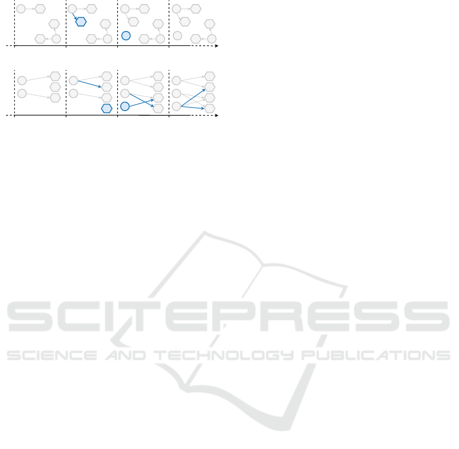
Figure 2(a) illustrates this network. The initial

graph G

dev,i

has nodes V = {p

, p

}, i.e.,

two players and three courses. The corresponding

edges are E

dev

= {(p

),(p

)}, deﬁning

the courses shared by each player. In G

dev,i+1

, player

shares a new course c

. In G

dev,i+2

, there appears

a new player p

without sharing any course. At last,

in G

dev,i+3

, nothing changes. Thus, the network can

only grow over time.

Besides creating new courses, a player can also

star courses of others players in SMM. In this sense,

the SMM network has also another directed bipartite

graph G

star

= {V,E

star

} with edges e ∈ E

star

of play-

ers p ∈ V that give stars to courses c ∈ V . Note that

the nodes in V are the same for both graphs G

dev,i

and

star,i

, considering a time instant t

. Similarly to graph

dev

, graph G

star

is also a dynamic network.

Figure 2(b) illustrates this network. In time t

graph G

star,i

has nodes V = {p

, p

} and

edges E

star

= {(p

),(p

)} indicating players

that starred courses. In G

star,i+1

, player p

stars

ICEIS 2019 - 21st International Conference on Enterprise Information Systems

p1 c3

p2

c1

c2

c4 c4

p3 p3

Gdev

Time

ti ti+1 ti+2 ti+3

p1 c3

p2

c1

c2

p1 c3

p2

c1

c2

c4

p1 c3

p2

c1

c2

(a) Graph G

dev

= {V,E

dev

}

p1

c1

p2

c2

c3

Time

ti ti+1 ti+2

c4

p3

c4

p3

c4

Gstar

ti+3

p1

c1

p2

c2

c3

p1

c1

p2

c2

c3

p1

c1

p2

c2

c3

(b) Graph G

star

= {V,E

star

}

Figure 2: Graphs G

dev

and G

star

changing over time.

course c

, and there appears a new course c

with no

star. In G

star,i+2

, there appears a new player p

that

stars course c

; also, player p

stars course c

. At

last, in G

star,i+3

, player p

stars courses c

and c

According to this discussion, the SMM game can

be represented by two dynamic networks, G

dev

and

star

, whose topologies are correlated and evolve as a

function of time. To analyze such correlated evolution

is essential when spotting game inﬂuencers, since the

courses that they develop become popular right after

they advertise them in other media, like Twitch and

YouTube, while the other players’ courses gain pop-

ularity gradually. The correlated evolution is proba-

bly even more important than looking for static graph

topologies in individual time stamps. With that in

mind, the main problem that we tackle in this paper

is: how to spot game inﬂuencers by evaluating the

correlated evolution of graphs G

dev

and G

star

Obviously, there exist other types of interactions

that lead to additional dynamic networks describing

the SMM game, such as, play, break time record, etc.

Nevertheless, without loss of generality, we only con-

sider G

star

and G

dev

in this paper, and show that they

are enough to accurately identify game inﬂuencers.

The next section describes existing works focused

on identifying inﬂuencer users in social networks.

3 INFLUENCER DETECTION

To the best of our knowledge, there is no research on

detecting inﬂuencers in Social Networks of Games;

the existing approaches to detect inﬂuencers in other

types of social networks are thus the closest related

works. In this section, we outline the state-of-the-art.

The na

ıve approaches to detect digital inﬂuencers

are based on selecting the top-ranked nodes identi-

ﬁed by some centrality indices; more advanced strate-

gies are greedy methods and heuristic methods (Wang

et al., 2017; Al-Garadi et al., 2018). The centrality-

based methods ﬁnd a set of the most inﬂuential nodes

based on the network topology (Barab

asi and P

osfai,

2016). In (Morone et al., 2016), it is presented an al-

gorithm that ranks nodes based on collective inﬂuence

propagation, which quantiﬁes the nodes’ “inﬂuences”

in the network. Meanwhile, another research infers

the inﬂuential nodes based on spreading paths (i.e.,

the links) (Wang et al., 2017).

Unfortunately, these algorithms work only on ho-

mogeneous networks (i.e., a single type of node),

while our problem refers to heterogeneous/bipartite

networks (i.e., nodes of two types, players and

courses). Also, we need to correlate two dynamic net-

works, and analyze their evolution over time. In this

sense, it is difﬁcult to use centrality indices because

they infer knowledge only based on the topology of

a single static network. To tackle our problem, one

must observe the nodes’ features, so to model game

inﬂuencers’ characteristics instead of ranking them.

In (Chino et al., 2017), a dynamic graph of com-

ments and online reviews was analyzed to detect sus-

picious users, like spammers. The authors model the

temporal aspect of the volume of activity (e.g., num-

ber of characters in a review) to detect an anomaly in

a social media. The proposed temporal aspect mod-

eling is interesting and inspiring, but this research

works with only one dynamic network and speciﬁc

application-related features of the contents, besides

detecting suspicious users; not, inﬂuential users.

Other approaches extract features to describe so-

cial media users; then, they use the features to train

Machine Learning (ML) algorithms to identify the

most inﬂuential ones. ML-based approaches have

great potential to identify inﬂuential users in large net-

works and complex networks (Al-Garadi et al., 2018).

In (Liu et al., 2014), temporal features are extracted

based on microblog posts (post-features) to train an

ML method to identify inﬂuential users in a tempo-

ral microblog network. The authors infer features for

a user according to his/her number of followers, the

number of microblog posts, the number of responses

received and the number of comments over time.

In (Qi et al., 2015), the aforementioned work is

extended by identifying domain-topics of inﬂuential

users so to improve the microblog’s search engines.

The improved work uses temporal post-features com-

bined with microblog text to ﬁt the domain-topics of

each inﬂuential user. Unfortunately, both works (Liu

et al., 2014) and (Qi et al., 2015) use a single dynamic

graph and heavily depend on the post-features, so it is

not clear how to use them to tackle our problem.

Finally, let us summarize the state-of-the-art on

inﬂuencer detection. Some techniques use central-

Detecting Inﬂuencers in Very Large Social Networks of Games

ity metrics to rank inﬂuential users based on graph

topology (Morone et al., 2016; Wang et al., 2017).

Other methods are designed to work with dynamic

networks; they commonly perform feature extraction

from the network and from the users’ external con-

tents to train ML algorithms (Liu et al., 2014; Qi

et al., 2015). Also, user modeling based on temporal

aspects has been applied (Chino et al., 2017). How-

ever, these works cannot tackle our problem mainly

because they do not correlate more than one dynamic

network and/or fail to quantify the changes/evolution

over time. In the next section, we present a novel

framework to tackle the problem.

4 PROPOSED METHODOLOGY

This section presents a new framework to detect inﬂu-

encers in very large Social Networks of Games. The

main question here is: how to model the correlated

evolution of players’ actions on the dynamic networks

dev

of developers and G

star

of stars? To answer it,

we propose a new player modeling heuristic based on

temporal aspects of their courses by extracting fea-

tures from the history of players’ actions over time.

4.1 Main Idea

Individually, neither network G

dev

nor G

star

has in-

trinsic characteristics that are truly useful to spot

game inﬂuencers. For example, by using an outdegree

centrality ranking algorithm on G

dev

we simply rank

the players by the number of shared courses; note that

it does not help much. Similarly, network G

star

would

lead to a ranking of players by the number of stars

given, which does not help either. Both rankings fail

to present relevant characteristics of the players that

would help identifying the inﬂuencers. Unfortunately,

the same problem happens when using more elabo-

rated analytical techniques, simply because there is

not enough information in any of the networks alone;

they must be analyzed combined.

As it was described before, we need to capture

relevant information from the correlated evolution of

both G

dev

and G

star

over time. To make it possible,

we propose to model this correlated evolution using

data streams, and to extract relevant features from the

streams to be used by a classiﬁcation ML algorithm.

4.2 Stream Modeling

In this sense, we obtain from G

star

the quantity ε

stars received by each course c by applying degree

centrality g(c) | c ∈ V in each instant of time t

. Thus,

a course is represented here by a stream of star count-

ing events c = [ε

,ε

,. ..], where each event ε

refers

to a pair (star

) with a number of stars star

and

a time stamp t

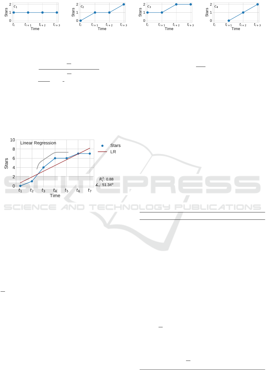
. Figure 3 illustrates this idea for the

toy graph G

star

shown in Figure 2(b). The number of

stars is constant over time for course c

, as it is shown

in Figure 3(a). Course c

received one star from p

time t

i+1

, and another one from p

in time t

i+3

(Figure

3(b)). Course c

received one star from p

in time t

i+2

(Figure 3(c)). At last, course c

received a new star in

each time instant after it arises in time t

i+1

(Figure

3(d)).

In this way, each course has a star counting stream

through time instants T = [t

,. ..]. In addition,

by observing G

dev

, for each player p its elaborated

courses are extracted, so C

= {c

,. ..}. There-

fore, we have for each player p a set C

of elaborated

courses and their stars counting stream over time.

Now, we need to extract temporal features from

each player. Note that each player p develops courses

c ∈ C

, and each course c has a star counting stream.

Thus, how to model the players based on their

courses? To accomplish this goal, we extract tem-

poral features of the courses and ensemble them to

model the players, as it is detailed in the next section.

4.3 Temporal Feature Extraction

This section describes our temporal aspects mod-

els. We developed three temporal features extractors.

Each extractor captures a speciﬁc characteristic of the

star counting stream. They use the players’ courses

and their stars counting streams to infer the features.

4.3.1 Linear Regression (LR)

The ﬁrst feature extractor, called Linear Regression

(LR) extractor, infers features related to the stars as-

cension of the courses, i.e., the growth of star count-

ing over time. The linear regression model is widely

used in social sciences; it can model the statistical re-

lation between the variables.

We used the well-known Least Squares method

for estimating the unknown parameters in the linear

model. Since each event ε

in the stream has only two

attributes (i.e., stars

and t

), the linear function can

be simpliﬁed to a vector (α,β) (Equation 1).

f (t

) = α + β ·t

= (α, β) (1)

In this sense, f (t

) represents an estimated star

counting for time t

. The parameters (α, β) are in-

ferred by the stars stream c = [ε

,ε

,. ..]. Considering

that stars is the average number of stars and t is the

average time, the parameters are deﬁned as follows:

ICEIS 2019 - 21st International Conference on Enterprise Information Systems

(a) c

stream (b) c

stream (c) c

stream (d) c

stream

Figure 3: Stream Modeling on the toy graph G

star

shown in Figure 2(b).

β =

∑

stars

−

|c|

∑

stars

∑

−

|c|

(

∑

)

α = stars − β ·t

(2)

Figure 4 illustrates an example of linear regres-

sion for a star counting stream c = [0, 1,4, 6,6,7,7]

between time instants t

and t

. The LR extractor ﬁnds

the linear function and extracts the angle ]

and the

coefﬁcient of determination R

of the course c. In this

example, ]

= 51.34

and R

= 0.88.

curvature

Figure 4: Linear Regression for a star counting stream.

The angle ]

represents how ascending are the

events of a star counting stream c. Meanwhile, the co-

efﬁcient of determination R

is the proportion of the

variance from the linear regression prediction, rang-

ing from 0 to 1. In this range, R

= 1 is the best pre-

diction for a stream c. The extractor uses coefﬁcient

to estimate a “curvature” on the stream; low R

represents how large the “curvature” is.

The LR extractor is in Algorithm 1. It infers for

each player’s course c ∈ C

(Line 8) the linear func-

tion model

, angle ]

and coefﬁcient of determination

(Line 9). In addition, the average angle coefﬁcient

] (Line 15) and the corresponding standard deviation

]

(Line 16) are extracted from the player’s courses.

How ascending is each player p? We measure the

angle ]

(Line 14) of a player p by the average vector

model

(Line 13) of the linear function of the courses

(Equation 3):

model

∑

c∈C

model

]

= angle(model

)

(3)

Additionally, it measures the entropy S

]

courses’ angles (Line 17). Entropy is a measure of

the randomness in the information, ranging from 0 to

∞ as the randomness increases. Thus, entropy veri-

ﬁes the tendency of player’s courses to have similar

ascension patterns, i.e., similar angles.

In Line 18, it is obtained the bottom-L lower co-

efﬁcients of determination R

of the courses, repre-

sented by R

rank

= [min

),. ..,min

)]. Also, the

top-L great angle ]

of courses is computed in Line

19, represented by ]

rank

= [max

(]),. ..,max

(])].

Thus, the extractor uses a parameter L ∈ N to deter-

mine the top-L and bottom-L.

Note the algorithm captures the bottom-L lower

coefﬁcients of determination R

rank

to identify “cur-

vatures”, whereas top-L angles ]

rank

to represent the

greatest star counting stream of a player.

Algorithm 1: LR Extractor.

1: procedure LR-MAP(c)  Course Modeling

2: model

← LinearRegression(c)

3: ]

← angle(model

)

4: R

← R

(model

,c)

5: return model

, ]

, R

6: procedure LR(p,L)  Player Modeling

7: Initialize models, ], R

with

8: for c ∈ C

9: model

, ]

, R

← LR-MAP(c)

10: models ← models ∪ {model

}

11: ] ← ] ∪ {]

}

12: R

← R

∪ {R

}

13: model

← mean(models)

14: ]

← angle(model

)

15: ] ← mean(])

16: σ

]

← std(])

17: S

]

← entropy(])

18: R

rank

← bottom(R

,L)

19: ]

rank

← top(], L)

20: return ]

, ], σ

]

rank

Detecting Inﬂuencers in Very Large Social Networks of Games

4.3.2 Delta Rank (DR)

The Delta Rank (DR) extractor infers features related

to star counting differences in time. The difference

∆ ∈ N between two sequential events ε

,ε

i+1

is:

∆ = stars

i+1

− stars

(4)

∆ means how many new stars a course c received

in a short temporal interval t

i+1

− t

. In this way, a

set D of star counting differences is extracted for a

course c, so D = {∆

,∆

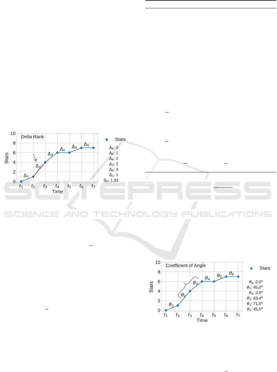
,. ..}. Figure 5 illustrates this

idea. Course c has six pairs of sequential events, so

D = {∆

,. ..,∆

} with the values 1, 3,2,0,1 and 0, re-

spectively. By ranking the values in D it is possible

to identify the greatest ∆; it is ∆

= 3 in this example.

Also, we measure the entropy S

of D values. In this

example, it is S

= 1.33.

greatest value

Figure 5: Delta Rank for a star counting stream.

The DR extractor is in Algorithm 2. It represents a

player p as the union of D for all its courses (Line 12),

so D

= D

∪ ... ∪ D

. A set S

of entropy values

for the courses (Line 13) is also collected. Then

we use D

and S

to infer features for player p.

In this analysis, we compute: ∆ that is the av-

erage of D

values (Line 14); σ

∆

that is the cor-

responding standard deviation (Line 15), and; S

∆

that is the entropy of D

values (Line 16). Also,

the extractor obtains the top-L great star count-

ing differences ∆ of the player, represented by

∆

rank

= [max

(∆),. ..,max

(∆)] (Line 17).

Additionally, the extractor analyzes the entropy

values S

of the player’s courses. It calculates the

average entropy

S of the courses (Line 18), and

the corresponding standard deviation σ

(Line 19).

Also, the extractor obtains the top-L great entropy

values S

of the player’s courses, represented by

rank

= [max

),. ..,max

)] (Line 20).

4.3.3 Coefﬁcient of Angle (CA)

The Coefﬁcient of Angle (CA) extractor infers fea-

tures related to the angles between events. The angle

θ between two sequential events ε

,ε

i+1

is:

Algorithm 2: DR Extractor.

1: procedure DR-MAP(c)  Course Modeling

2: Initialize D with

3: for i ← 1 to |c| − 1 do

4: ∆ ← stars

i+1

− stars

5: D ← D ∪ {∆}

6: S

← entropy(D)

7: return D, S

8: procedure DR(p,L)  Player Modeling

9: Initialize D

, S

with

10: for c ∈ C

11: D, S

← DR-MAP(c)

12: D

← D

∪ D

13: S

← S

∪ {S

}

14: ∆ ← mean(D

)

15: σ

∆

← std(D

)

16: S

∆

← entropy(D

)

17: ∆

rank

← top(D

,L)

18: S ← mean(S

)

19: σ

← std(S

)

20: S

rank

← top(S

,L)

21: return ∆, σ

∆

, S

∆

, ∆

rank

, S, σ

, S

rank

θ = tan

−1

∆

i+1

−t

(5)

θ means the star counting ascension between an in-

terval t

i+1

− t

. For each course, it is extracted a set

T = {θ

,θ

,. ..} of coefﬁcients of angle. Note that θ

varies within interval [0

,90

); high values indicate

high star counting growth in two sequential events.

Figure 6 illustrates this idea. Course c has six pairs

of sequential events, so T = {θ

,. ..,θ

} with values

45.0

,71.6

,63.4

,0.0

,45.0

and 0.0

, respectively.

high grown

Figure 6: Coefﬁcient of Angle for a star counting stream.

The CA extractor is in Algorithm 3. It represents a

player p as the union of T for all its courses (Line 12),

so, T

= T

∪ ... ∪ T

. Then it analyzes T

to infer

features for player p.

In the analysis, we obtain: θ that is the average

of values in T

(Line 13), and; σ

that is the corre-

ICEIS 2019 - 21st International Conference on Enterprise Information Systems

sponding standard deviation (Line 14). We also cal-

culate the player’s top-L high growth θ, represented

as θ

rank

= [max

(θ),. ..,max

(θ)] (Line 15).

Algorithm 3: CA Extractor.

1: procedure CA-MAP(c)  Course Modeling

2: Initialize T with

3: for i ← 1 to |c| − 1 do

4: ∆ ← stars

i+1

− stars

5: θ ← tan

−1

(∆)/(t

i+1

−t

)

6: T ← T ∪ {θ}

7: return T

8: procedure CA(p,L)  Player Modeling

9: Initialize T

with

10: for c ∈ C

11: T ← CA-MAP(c)

12: T

← T

∪ T

13: θ ← mean(T

)

14: σ

← std(T

)

15: θ

rank

← top(T

,L)

16: return θ, σ

, θ

rank

4.3.4 The F

ALL

Feature Extractor

Each feature extractor, i.e., LR, DR, and CA, infers a

series of features for a player p. They are then com-

bined into a single feature extractor F

ALL

(p,L) = LR(p,L) + DR(p,L) +CA(p,L) (6)

The three feature extractors have an input param-

eter L ∈ N that determines the quantity of ranked val-

ues to be extracted, each one with its particularities.

Note that, whenever L exceeds the number of values

available to rank some characteristic of a player, the

missing values are assumed to be zeros.

4.4 Framework

This section summarizes our proposed strategy to de-

tect game inﬂuencers in Social Networks of Games.

Given the actions of millions of players in an online

game, how to detect the game inﬂuencers? It is ob-

viously necessary to model the players’ characteris-

tics, but how can it be done? So far we have no-

ticed that neither graph G

dev

nor G

star

has intrinsic

characteristics that are truly useful to spot game in-

ﬂuencers, since we need to capture relevant informa-

tion from the correlated evolution of both graphs over

time. Then, we described how to model this corre-

lated evolution using data streams, from which we ex-

tract relevant features that properly represent the play-

ers’ characteristics. Now, we propose to simply ex-

press the game inﬂuencer detection problem as a clas-

siﬁcation ML task, using the features of our extractors

as input. In the next section, we validate our proposal

with the famous SMM game; speciﬁcally, we report

experimental results to show that our framework de-

tects game inﬂuencers of different nations with high

accuracy.

5 EXPERIMENTS

We performed a series of experiments to validate our

proposal. They are described in the following:

1. In the ﬁrst experiment, we analyzed each feature

extractor individually, considering players from

one country only, i.e., Canada;

2. In the second experiment, we analyzed the ensem-

ble of the three feature extractors, also consider-

ing Canadian players.

3. We then performed input parameter tuning in the

classiﬁers to improve their results.

4. At last, we validated the best classiﬁer on data

from another country, i.e., France, so to demon-

strate the generality of our framework.

In the ﬁrst two experiments, we applied a set of 28

classiﬁcation algorithms. They are: AdaBoostClas-

siﬁer, BaggingClassiﬁer, BernoulliNB, Calibrated-

ClassiﬁerCV, ComplementNB, DecisionTreeClassi-

ﬁer, ExtraTreeClassiﬁer, ExtraTreesClassiﬁer, Gaus-

sianNB, GaussianProcessClassiﬁer, GradientBoost-

ingClassiﬁer, KNeighborsClassiﬁer, LinearDiscrim-

inantAnalysis, LinearSVC, LogisticRegression, Lo-

gisticRegressionCV, MLPClassiﬁer, MultinomialNB,

NearestCentroid, NuSVC, PassiveAggressiveClas-

siﬁer, Perceptron, QuadraticDiscriminantAnalysis,

RandomForestClassiﬁer, RidgeClassiﬁer, RidgeClas-

siﬁerCV, SGDClassiﬁer, and SVC.

The algorithms are implemented in Python 3 with

the sklearn package. We used the standard input pa-

rameter values of each algorithm. For reproducibility,

our code is open-sourced at GitHub

, We present how

to use it and the performed experiments.

5.1 Dataset Collection

We crawled data from the Super Mario Maker game

on the SMM Bookmark website

continuously over

GitHub. “Detecting Inﬂuencers in Very Large SNG”

https://github.com/leomaurodesenv/paper-2019-iceis

SMM Bookmark. https://supermariomakerbookmark.

nintendo.net (accessed December 03, 2018).

Detecting Inﬂuencers in Very Large Social Networks of Games

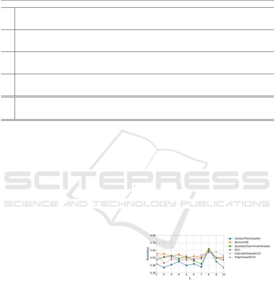
Table 2: Experiments: results of the top-3 best classiﬁers in each experiment.

Algorithm Accuracy Precision Recall F1-score

DecisionTreeClassiﬁer 0.670 (±0.079) 0.621 (±0.109) 0.645 (±0.100) 0.595 (±0.100)

BernoulliNB 0.665 (±0.106) 0.432 (±0.145) 0.600 (±0.100) 0.489 (±0.131)

QuadraticDiscriminantAnalysis 0.665 (±0.106) 0.432 (±0.145) 0.600 (±0.100) 0.489 (±0.131)

DecisionTreeClassiﬁer 0.690 (±0.065) 0.680 (±0.089) 0.658 (±0.070) 0.632 (±0.073)

ExtraTreeClassiﬁer 0.670 (±0.067) 0.616 (±0.101) 0.653 (±0.075) 0.607 (±0.087)

GradientBoostingClassiﬁer 0.670 (±0.055) 0.593 (±0.102) 0.613 (±0.058) 0.579 (±0.077)

GradientBoostingClassiﬁer 0.740 (±0.069) 0.745 (±0.068) 0.766 (±0.076) 0.722 (±0.072)

BaggingClassiﬁer 0.696 (±0.090) 0.648 (±0.104) 0.675 (±0.106) 0.640 (±0.096)

ExtraTreeClassiﬁer 0.680 (±0.071) 0.650 (±0.086) 0.687 (±0.091) 0.644 (±0.079)

ALL

LogisticRegression 0.808 (±0.108) 0.808 (±0.108) 0.733 (±0.157) 0.745 (±0.142)

RidgeClassiﬁerCV 0.775 (±0.105) 0.733 (±0.131) 0.675 (±0.155) 0.685 (±0.144)

LinearSVC 0.750 (±0.113) 0.750 (±0.111) 0.683 (±0.154) 0.688 (±0.139)

Tuning

LogisticRegression 0.8709 (±0.066) 0.9029 (±0.053) 0.8588 (±0.080) 0.8573 (±0.076)

RidgeClassiﬁerCV 0.8064 (±0.220) 0.7903 (±0.270) 0.8225 (±0.212) 0.7849 (±0.255)

LinearSVC 0.8387 (±0.094) 0.8596 (±0.097) 0.8306 (±0.103) 0.8266 (±0.099)

a three-months period, collecting information about

74,915 courses, and 884,302 players in which 32,055

are makers (i.e., players who elaborated courses).

These courses were developed by Canadian and

French makers and received more than 380,000 stars.

The data was split into Canadian makers (CAN

dataset) that elaborated 34,479 courses, and French

makers (FRA dataset) that elaborated 40,436 courses.

The idea is to use the CAN dataset in a train/test step,

and the FRA dataset in a validation step.

To make it possible, we had to create ground truth

for the CAN dataset. Speciﬁcally, we ﬁrst ranked the

top-100 makers from CAN dataset based on the total

count of stars received by all of their courses. In this

sense, we selected graph G

star, f

of the last timestamp

to get the degree centrality (Barab

asi and P

osfai,

2016, ch.2) of each course , so it is the stars counting

of course c in G

star, f

. Also, graph G

dev, f

was used to

identify the maker’s courses.

Then, we manually labeled the top-100 makers

into two classes, non-inﬂuencer and inﬂuential player,

by checking their social activities searching the Web

with Google and also sites of the communities of

games. In total, 41% (41) inﬂuential and 59% (59)

non-inﬂuencer players were identiﬁed.

Our consensus to determine whether a player is an

inﬂuencer is if the player markets/publish its courses

in popular sites of the communities of SMM, they

are: Reddit, GameFAQs, Twitch, YouTube, Face-

book, NintendoLife, and Makers of Mario.

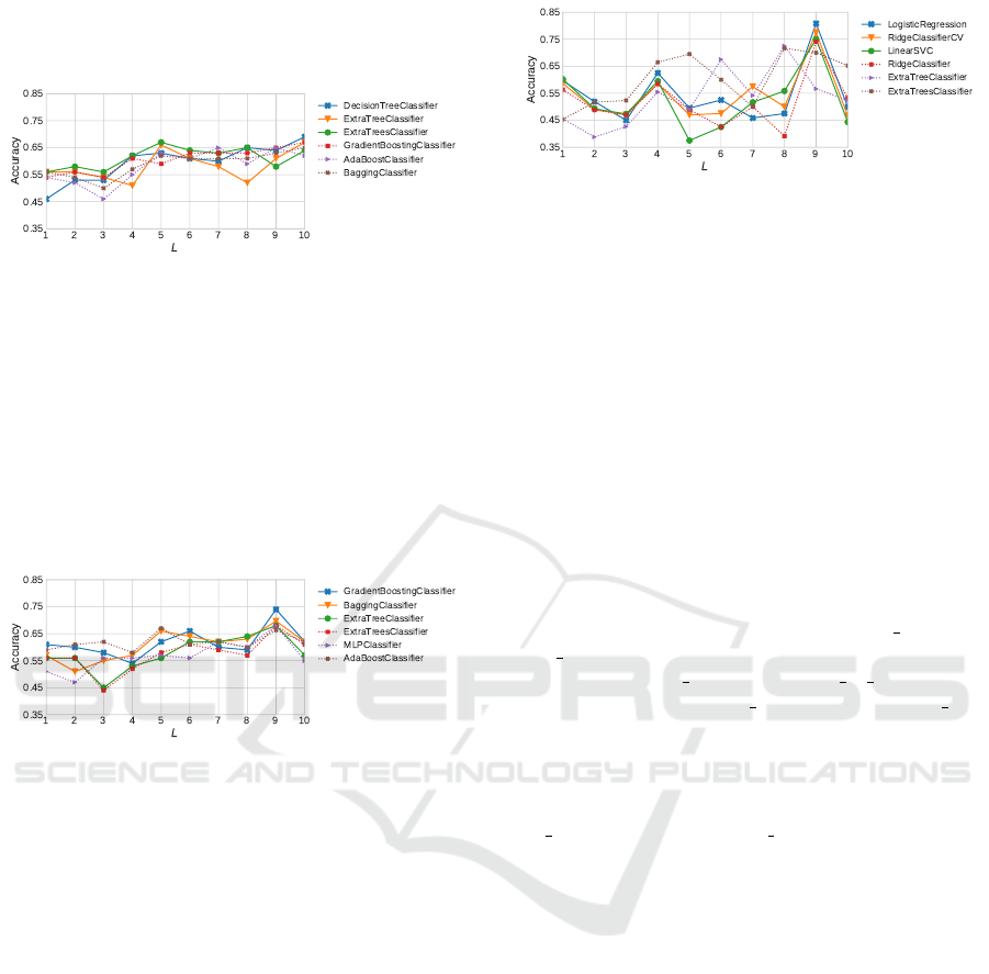
5.2 Feature Extractors Experiments

In the ﬁrst experiment, we evaluated each feature ex-

tractor individually, i.e., LR, DR and CA. Here, the

CAN dataset was used with a 5-fold cross-validation

strategy. We evaluated the LR extractor with L rang-

ing from 1 to 10. Figure 7 reports accuracy results

for the top-6 classiﬁers. In this interval, the LR

(L = 8) extracting 20 attributes presented the best av-

erage accuracy. The results of the best classiﬁers for

the LR extractor (L = 8) are shown in Table 2. The

DecisionTreeClassiﬁer algorithm had the best perfor-

mance with accuracy of 67.0% and f1-score of 59.5%.

Figure 7: Accuracy of the top-6 classiﬁers using the LR

feature extractor with parameter L ranging from 1 to 10.

Figure 8 reports the accuracy of the top-6 classi-

ﬁers using the DR extractor with L ranging from 1

to 10. First, we observe that the average accuracy

of classiﬁers grows with L. However, if L becomes

higher than the number of values ranked, nonexistent

attributes will be ﬁlled with zeros. In this sense, L

cannot be so great. Second, the experiment shows

that L = 10 present the best average accuracy with

25 attributes. Table 2 reports the evaluation of the 3

best classiﬁers for the DR extractor (L = 10). The De-

ICEIS 2019 - 21st International Conference on Enterprise Information Systems

100

cisionTreeClassiﬁer had the best performance again,

with 69.0% accuracy and 63.2% f1-score.

Figure 8: Accuracy of the top-6 classiﬁers using the DR

feature extractor with parameter L ranging from 1 to 10.

At last, we evaluated the CA extractor with L rang-

ing from 1 to 10. Figure 9 reports results from the

top-6 classiﬁers with the highest accuracy. The best

average accuracy was obtained with L = 9, using 11

attributes only. The results of the 3 best classiﬁers

for the CA extractor (L = 9) are shown in the Ta-

ble 2. Here, we highlight the GradientBoostingClas-

siﬁer with 74.0% accuracy and 72.2% f1-score.

Figure 9: Accuracy of the top-6 classiﬁers using the CA

feature extractor with parameter L ranging from 1 to 10.

In summary, the three feature extractors presented

average results in a classiﬁcation task, with approxi-

mately 70% accuracy.

5.3 Framework Experiments

In this section, we analyze the F

ALL

feature extractor,

i.e., the ensemble of the three feature extractors that

we proposed. Once more, we used the CAN dataset

with a 5-fold cross-validation strategy.

Figure 10 reports the accuracy of the top-6 classi-

ﬁers using F

ALL

with L ranging from 1 to 10. In this

experiment, L = 9 clearly leads to the best average

accuracy, using 56 attributes. Table 2 reports results

for the 3 best classiﬁers with F

ALL

extractor (L = 9).

We highlight the LogisticRegression with the 80.8%

accuracy and 74.5% f1-score.

Note that the framework F

ALL

presented better re-

sults than the feature extractors individually. In addi-

tion, the top algorithms that were similar to the feature

extractors also changed, as well as the performance of

the LogisticRegression. F

ALL

(L = 9) presented great

Figure 10: Accuracy of the top-6 classiﬁers using the F

ALL

feature extractor with the L ranging from 1 to 10.

results using 56 attributes, meanwhile the LR (L = 8),

DR (L = 10) and CA (L = 9) used 20, 25 and 11 fea-

tures, respectively. However, LogisticRegression us-

ing F

ALL

(L = 9) obtained the best accuracy (80.8%),

precision (80.8%), and f1-score (74.5%).

5.4 Parameter Tuning

In this step, we focused on improving the top-3 classi-

ﬁers of the framework experiments (F

ALL

(L = 9)) us-

ing a grid search, that is, an exhaustive search through

the hyperparameter space of the classiﬁers.

The grid search on each classiﬁer’s parameters,

i.e., LogisticRegression (C, dual, f it intercept,

max iter, penalty, solver), RidgeClassiﬁerCV

(al phas, cv, f it intercept, store cv values) and

LinearSVC (C, dual, f it intercept, loss, max iter,

penalty), also used the CAN dataset with a 5-fold

cross-validation strategy.

Table 2 reports the best results of each classi-

ﬁer. The LogisticRegression (C = 0.9, dual = True,

f it intercept = True, max iter = 100, penalty =

l2, solver = warn) using F

ALL

(L = 9) obtained the

best accuracy (87.1%), precision (90.3%), recall

(85.9%), and f1-score (85.7%). The performance of

RidgeClassiﬁerCV and LinearSVC also improved.

5.5 Validation

The validation experiment evaluated the generality of

our framework. Here, we used the best conﬁguration,

i.e., F

ALL

(L = 9) plus LogisticRegression with the

ﬁne tuned parameter values of Section 5.4, taking the

whole CAN dataset for training and the FRA dataset

for testing. At ﬁrst, we ranked the top-100 makers

from the FRA dataset based on their total number of

stars received. Then, we used F

ALL

(L = 9) to infer the

players’ features and the LogisticRegression classiﬁer

to label the game inﬂuencers. Thanks to our proposed

framework, the algorithm labeled 27 players as game

inﬂuencers, automatically, in which 21 were manu-

ally conﬁrmed as true inﬂuencers. Thus, our proposed

model presented 77.8% precision to ﬁnd inﬂuencers

Detecting Inﬂuencers in Very Large Social Networks of Games

101

with a classiﬁer trained in data from another coun-

try. These results indicate that our proposal is generic

enough to accurately model the behaviour of game in-

ﬂuencers from different nationalities.

6 CONCLUSION

This paper presented a novel framework to detect

game inﬂuencers in Social Networks of Games.

Given the actions of millions of players in an online

game, how to detect the most inﬂuential users? It was

obviously necessary to model the players’ character-

istics, but how can it be done? To tackle the prob-

lem, we needed to capture relevant information from

the correlated evolution of more than one dynamic

network over time, which could not be performed

with the existing works. Then, we described how

to model this correlated evolution using data streams,

from which we extracted relevant features to properly

represent the players’ characteristics, and mapped the

game inﬂuencer detection problem into a classiﬁca-

tion ML task that uses our features as input. Finally,

we validated our proposal by studying the famous Su-

per Mario Maker game, from Nintendo Inc., Japan.

The novel framework includes three feature ex-

tractors, i.e., Linear Regression, Delta Rank and Co-

efﬁcient of Angle. They are unsupervised and based

on the temporal aspects of the players’ actions on

the social network. In the experimental evaluation,

28 classiﬁcation algorithms were studied. Using our

features as input, the LogisticRegression classiﬁer ob-

tained the bests results with accuracy (87.1%), preci-

sion (90.3%), recall (85.9%) and f1-score (85.7%).

We also demonstrated that the proposed framework

automatically detects game inﬂuencers with high ac-

curacy even when using data from distinct nations for

testing and training.

Analyzing Other Types of Social Networks: in

theory, our methodology can also be used in non-

game-related applications, such as to spot inﬂuencers

in other types of social networks by analyzing the

“likes” received by posts over time. Minor adapta-

tions may be needed, due to domain speciﬁcities. Ba-

sically, two dynamic networks are the only require-

ment; one to store the creator of digital content and

another to represent positive reactions (e.g., “like”) of

users to the content, as it is formalized in the paper.

Further Research: (1) analyze inﬂuencers’

games to discover popular games’ characteristics,

e.g., platform games’ characteristics, such as general

monsters, course size, challenges, traps, and so on;

(2) apply this framework in other domains to spot in-

ﬂuencers; (3) also, use regression modeling to study

different degrees of inﬂuence over the players.

ACKNOWLEDGEMENTS

This work was supported by the Brazilian National

Council for Scientiﬁc and Technological Develop-

ment (CNPq); Coordination for the Improvement of

Higher Education Personnel - Brazil (CAPES) [grant

001]; Sao Paulo Research Foundation (FAPESP)

[grant 2018/05714-5]; and AWS Cloud Credits for

Research.

REFERENCES

Al-Garadi, M. A., Varathan, K. D., Ravana, S. D., Ahmed,

E., Mujtaba, G., Khan, M. U. S., and Khan, S. U.

(2018). Analysis of online social network connections

for identiﬁcation of inﬂuential users: Survey and open

research issues. ACM Comput. Surv., 51(1):16:1–

16:37.

Barab

asi, A.-L. and P

osfai, M. (2016). Network science.

Cambridge university press, Cambridge, USA.

Chino, D. Y. T., Costa, A. F., Traina, A. J. M., and Falout-

sos, C. (2017). VolTime: Unsupervised Anomaly De-

tection on Users’ Online Activity Volume, pages 108–

116. SIAM International Conference on Data Mining.

Gros, D., Hackenholt, A., Zawadzki, P., and Wanner, B.

(2018). Interactions of twitch users and their usage

behavior. In Meiselwitz, G., editor, Social Computing

and Social Media. Technologies and Analytics, pages

201–213, Cham. Springer International Publishing.

Hilvert-Bruce, Z., Neill, J. T., Sj

oblom, M., and Hamari, J.

(2018). Social motivations of live-streaming viewer

engagement on twitch. Computers in Human Behav-

ior, 84:58 – 67.

Kamber, M., Han, J., and Pei, J. (2012). Data mining: Con-

cepts and techniques. Elsevier, Amsterdam.

Lee, J., Lee, M., and Choi, I. H. (2012). Social network

games uncovered: Motivations and their attitudinal

and behavioral outcomes. Cyberpsychology, Behav-

ior, and Social Networking, 15(12):643–648. PMID:

23020746.

Liu, N., Li, L., Xu, G., and Yang, Z. (2014). Identify-

ing domain-dependent inﬂuential microblog users: A

post-feature based approach. In AAAI, pages 3122–

3123.

Lucas, S. M. (2009). Computational intelligence and ai

in games: A new ieee transactions. IEEE Transac-

tions on Computational Intelligence and AI in Games,

1(1):1–3.

Morone, F., Min, B., Bo, L., Mari, R., and Makse, H. A.

(2016). Collective inﬂuence algorithm to ﬁnd inﬂu-

encers via optimal percolation in massively large so-

cial media. Scientiﬁc reports, 6:30062.

Pei, S., Morone, F., and Makse, H. A. (2018). Theories for

Inﬂuencer Identiﬁcation in Complex Networks, pages

125–148. Springer International Publishing, Cham.

ICEIS 2019 - 21st International Conference on Enterprise Information Systems

102

Qi, L., Huang, Y., Li, L., and Xu, G. (2015). Learning to

rank domain experts in microblogging by combining

text and non-text features. In 2015 International Con-

ference on Behavioral, Economic and Socio-cultural

Computing (BESC), pages 28–31.

Savi

c, M., Ivanovi

c, M., and Jain, L. C. (2019). Introduction

to Complex Networks, pages 3–16. Springer Interna-

tional Publishing, Cham.

oblom, M. and Hamari, J. (2017). Why do people watch

others play video games? an empirical study on the

motivations of twitch users. Computers in Human Be-

havior, 75:985 – 996.

Strang, G., Strang, G., Strang, G., and Strang, G. (2016).

Introduction to Linear Algebra, volume 5. Wellesley-

Cambridge Press Wellesley, MA.

Wang, X., Zhang, X., Yi, D., and Zhao, C. (2017). Identify-

ing inﬂuential spreaders in complex networks through

local effective spreading paths. Journal of Statistical

Mechanics: Theory and Experiment, 2017(5):053402.

Westaby, J. D. (2012). Dynamic network theory: How so-

cial networks inﬂuence goal pursuit. American Psy-

chological Association.

Yannakakis, G. N. and Togelius, J. (2015). A panorama

of artiﬁcial and computational intelligence in games.

IEEE Transactions on Computational Intelligence and

AI in Games, 7(4):317–335.

Yannakakis, G. N. and Togelius, J. (2018). Artiﬁcial Intelli-

gence and Games. Springer International Publishing,

Cham.

Detecting Inﬂuencers in Very Large Social Networks of Games

103