
Well Detection in Satellite Images using Convolutional Neural Networks
Pratik Sanjay Wagh, Debanjan Das
∗
and Om P. Damani
Department of Computer Science & Engineering, IIT Bombay, Mumbai, India
Keywords:
Remote Sensing, Computer Vision, Object Detection, Convolutional Neural Networks, Machine Learning.
Abstract:
The Government of India conducts a well census every five years. It is time-consuming, costly, and usually
incomplete. By using transfer learning-based object detection algorithms, we have built a system for the auto-
matic detection of wells in satellite images. We analyze the performance of three object detection algorithms -
Convolutional Neural Network, HaarCascade, and Histogram of Oriented Gradients on the task of well detec-
tion and find that the Convolutional Neural Network based YOLOv2 performs best and forms the core of our
system. Our current system has a precision value of 0.95 and a recall value of 0.91 on our dataset. The main
contribution of our work is to create a novel open-source system for well detection in satellite images and cre-
ate an associated dataset which will be put in the public domain. A related contribution is the development of
a general purpose satellite image annotation system to annotate and validate objects in satellite images. While
our focus is on well detection, the system is general purpose and can be used for detection of other objects as
well.
1 INTRODUCTION
Automation of well records promises to be a big
step in developing countries’ E-governance initia-
tives. Currently, the well census in India is conducted
every five years and in between, farmers are supposed
to contact the nearest revenue department office to get
their land records updated with their well informa-
tion. This is rarely done, especially due to complex
ownership issues. Many government schemes offered
to farmers are contingent upon the assets held by the
farmer, e.g. to qualify for the drip irrigation sub-
sidy, and farmers are unable to take benefit of these
schemes when records are not up-to-date.
Not just for individual farmers, but for the coun-
try as a whole, it is important to have good data on
groundwater use for planning and governance (Min-
istry of Water Resource, 2006a). For example, the
Central Groundwater Board estimates the country’s
net irrigated area and irrigation potential using the
well count and the counts of other ground and sur-
face water sources obtained through the minor irriga-
tion census. The process of estimating a watershed’s
groundwater development also requires the estimate
of groundwater use which uses the well count data.
There are several administrative and resource-
related challenges (Ministry of Water Resource,
∗
This author is also co-first author.
2006b) in conducting the well census. This surveying
process is time-consuming, lengthy, and cost ineffec-
tive due to which the collected data is often incom-
plete and potentially corrupt. As a first step towards
solving this problem, we exploit the recent advances
(Redmon et al., 2015; LeCun et al., 1999; Viola and
Jones, 2001; Dalal and Triggs, 2005; Albert et al.,
2017) in the area of applied machine learning and
computer vision, to automate the task of maintaining
well records. Later, we can overlay the cadastral maps
giving land ownership, with GIS maps with detected
wells, and classify well ownership by class, caste, re-
gions etc (Ministry of Water Resource, 2006c).
The task of automatic well detection is challeng-
ing since the actual real-life well looks quite different
from the wells present in satellite images. The con-
trast is depicted in Figure 2. This implies that object
detection methods that work well for real-life cam-
era images may not be suitable for object detection in
satellite images.
We observe that the wells in the Google Maps im-
ages are like dark circular shaped objects with a thin
white cyclic patch around it. A further challenge in
automatic well detection is that sizes of the wells in
developing countries are such that they generally look
very similar to tree or shadow of the trees (Figure 2),
and parts of the well maybe covered by the trees. This
poses challenge even for human annotators.
Wagh, P., Das, D. and Damani, O.
Well Detection in Satellite Images using Convolutional Neural Networks.
DOI: 10.5220/0007734901170125
In Proceedings of the 5th International Conference on Geographical Information Systems Theory, Applications and Management (GISTAM 2019), pages 117-125
ISBN: 978-989-758-371-1
Copyright
c
2019 by SCITEPRESS – Science and Technology Publications, Lda. All rights reserved
117
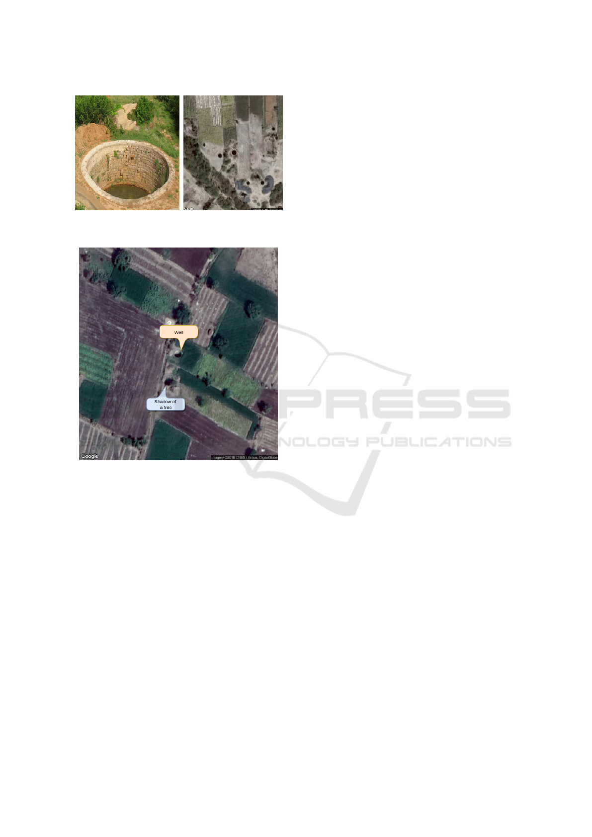
Figure 1: Contrast between real-life well and wells in satel-
lite images (Maitra, 2011).
Figure 2: Similarity between well and shadow of a tree in a
satellite image.
While the analysis of satellite imagery is quite an
old field, the application of deep learning in this area
is a new and emerging trend. Existing work in the area
focuses on detection of man-made objects in satellite
images, e.g, air-crafts(Wu et al., 2015), vehicles(Chen
et al., 2014) and oil tanks(Zhang et al., 2015). All of
these works follow a process pipeline approach. First,
the object is localized, then it is recognized, and then
the classification happens. The binarized normed gra-
dients (Cheng et al., 2014) is used in (Wu et al., 2015)
to localize the air-crafts present in a satellite image
and then a Hybrid Deep Convolutional Neural Net-
work is used for feature extraction, and for classifica-
tion support-vector machines (Vapnik, 1999) is used.
Similarly, in (Zhang et al., 2015), the object of in-
terest is oil-tanks, and hence the elliptical or circular
shapes in an image are detected using ellipse and line
segment detector. After object localization, they use
Histogram of Oriented Gradients (Dalal and Triggs,
2005) and Convolutional Neural Networks methods
for feature extraction.
All of these methods require large training sets.
In the area of urban planning where training data is
scarce, the concept of transfer learning is used in (Al-
bert et al., 2017) for object classification and feature
extraction.
In the context of general object detection algo-
rithms, we first worked with the basic Convolu-
tional Neural Network architectures (LeCun et al.,
1999), HaarCascade (Viola and Jones, 2001) and
Histogram of Oriented Gradients (Dalal and Triggs,
2005) with support-vector machine (Vapnik, 1999)
methods. However, we achieved limited success to-
wards well detection with these approaches.
Then, inspired by the success of transfer learn-
ing approach in urban planning context (Albert et al.,
2017), we decided to experiment with the transfer
learning technique in the context of rural planning.
We experimented with the popular single shot object
detection algorithms You Only Look Once (YOLOv2
(Redmon and Farhadi, 2016)). In this work, the prob-
lem of object detection is framed as a regression prob-
lem where it outputs the probable bounding box co-
ordinates and the class probabilities for each bound-
ing box. YOLO uses Deep Convolutional Neural Net-
works for image recognition and bounding box draw-
ing. In contrast to the pipeline approaches, it performs
the object detection in the single shot, which makes it
a lot faster than other object detection algorithms.
In the literature, several authors lament the
scarcity of good quality data for object detection in
satellite images and manually collect data from dif-
ferent sources. For our well detection problem also,
there is no existing satellite image dataset with wells
identified in it. As we collaborated with members of
the Rural Development Department for data collec-
tion, we realized the need for a proper system to an-
notate and validate wells in the satellite images. To
our surprise, no such system was available in the pub-
lic domain. Hence, we decided to develop a general
purpose satellite image annotation system (SIAS) us-
ing which one can annotate and validate objects of
any type in satellite images.
The contribution of our work is two-fold. The
main contribution of our work is to create a novel
open-source transfer learning based system for well
detection in satellite images and create an associated
dataset to be put in the public domain. A related
contribution is the development of a general purpose
satellite image annotation system to annotate and val-
idate objects in satellite images. While our focus is
on well detection, the system is general purpose and
can be used for detection of other objects as well.
GISTAM 2019 - 5th International Conference on Geographical Information Systems Theory, Applications and Management
118

In Section 2, we discuss our SIAS system. Section
3 describes the object detection algorithms which we
have used, in Section 4 we discuss about the dataset,
performance metric we used and the training proce-
dure we followed and the last section contains the
conclusions.
2 SYSTEM ARCHITECTURE
In addition to experimenting with machine learning
algorithms, it is important to build a system that is in-
tuitive to use for end users. In our case, end users will
be government officials who may not be very com-
puter savvy. Hence we developed a web-based ap-
plication that can be used across the internet. Further,
the same system should be capable of taking feedback
from the user where the user can validate or invalidate
the detected well. A user should also be able to mark
an undetected well. In fact, this feedback should flow
into the system and get added to the training set. This
way the training set will keep growing over time as the
system gets used. We call our system SIAS - Satellite
Image Annotation System.
The architecture diagram of the whole system is
given in Figure 3.
2.1 User Interface
We follow the Software As A Service (SaaS) model.
At the backend, we use Flask (Ronacher, 2010) which
is a micro-web framework. The frontend is developed
with HTML, CSS, and JavaScript. The user interface
is shown in Figure 4.
2.1.1 Frontend
The adoption of the system critically depends on the
user-friendliness of the frontend. Various features of
frontend are listed below.
• It contains a search bar and a map window where
one can search for a place and the resulting satel-
lite image is shown in that window.
• There is an optional field, using which we can se-
lect the model we want to use. The available mod-
els are YOLOv2, tinyYOLOv3, Basic Convolu-
tional Neural Network model, the Histogram of
Oriented Gradients-support-vector machines and
HaarCascade.
• After searching for a place and selecting the
model, clicking on ”Predict” button shows the
predicted wells in that area with the help of
bounding boxes. These bounding boxes are su-
perimposed on the satellite image.
• Note that user can select an arbitrarily large area
to predict. We subdivide the selected area into
multiple blocks of size 640 × 640. Each of these
blocks is then given as input to the selected model.
Currently, if a well falls on the boundary of two
sub-blocks then it is not detected. In the future,
we plan to solve this problem by creating differ-
ent partition sets of the same area and merging the
results from these partition sets.
• An important feature of the system is that it pro-
vides the user ability to give feedback. Each of the
predicted boxes can be marked as valid or invalid
by the user. This way the training set will keep
growing over time as the system gets used.
• The user can also label any object of interest in the
image by selecting and marking the correspond-
ing area.
2.1.2 Backend
The backend acts as a bridge between the object de-
tection models and frontend. Images from frontend
come in the form of a base64 string. In the backend,
it is decoded and converted into PNG images and the
model is applied to it. The output image is then sent
back to the frontend.
3 OBJECT DETECTION
ALGORITHMS
We experimented with various object detection meth-
ods and found that transfer learning based YOLO
model performs the best. We next describe the meth-
ods tried.
3.1 Basic Convolutional Neural
Network
In this model we have used CNN as a feature extrac-
tor and multi-layer perceptron (MLP) as a classifier.
We have created a two-layered Convolutional Neural
Network (CNN) model. The description of the model
is given as:
• The first convolutional stage is with rectified lin-
ear unit (ReLU) activation function followed by
a max-pooling layer. This layer has 20 convolu-
tional filters, each one of them has a size of 5 × 5.
The output dimension is the same as that of the
input shape i.e, 64 × 64. As this is the first layer
in our model, we have to define its input shape
i.e, (1,64,64). The max-pooling operation applies
a sliding window that slides over the image and
Well Detection in Satellite Images using Convolutional Neural Networks
119

Figure 3: SIAS system architecture.
Figure 4: User interface of the SIAS system.
takes the maximum value of the pixel present in
that region.
• The second convolutional layer is also followed
by rectified linear unit activation function and a
max-pooling layer. Now, we increase the number
of convolutional filters to 50 from 20 in the previ-
ous layer.
• Then we have a standard flattening layer and a
dense layer of 500 neurons. This flattening layer
flattens the last 3D feature block of the CNN and
provides it to the dense layer. This dense layer
acts as a hidden layer. The output layer of the
MLP has softmax function as activation function,
which can be defined as:
P(y = j|X) =
e
X
T
·w
∑
K
k=1
e
X
T
·w
GISTAM 2019 - 5th International Conference on Geographical Information Systems Theory, Applications and Management
120

where K is the number of classes and P(y = j|X)
is the probability of the input being in class j
given it’s feature vector X.
3.2 HaarCascade
Introduced in 2006, it has been very successful at
face detection problem(Viola and Jones, 2001). Since
then it has been used for various other object detec-
tion problems which use non-satellite images. It uses
the Haar-like feature for detecting an object. It has
introduced an integral image for efficient and quick
calculation of the sum of pixel values in a rectangular
subset of the given image, thus lowers the computa-
tion time. It uses AdaBoost classifier for classifying
the positive and negative feature.
3.3 HOG
Histogram of Oriented Gradient (HOG)(Dalal and
Triggs, 2005) is a feature descriptor method. This
method uses the orientation of an image as a feature
for detecting an object thus generalizes well for the
objects which have a fixed shape. It first divides the
image into small connected blocks which consist of
cells and then computes the histogram of the gradient
for each pixel within the cell. Then it discretizes each
cell into angular bins according to the gradient ori-
entation. Each cell is combined to form blocks, these
blocks are normalized and used as a feature descriptor
which is used with support-vector machine (Vapnik,
1999) for object detection.
3.4 YOLOv2
You Only Look Once (YOLOv2) (Redmon and
Farhadi, 2016) introduced in late 2016 gave a mean
Average Precision (mAP) of 76.8 on VOC 2007
dataset, is an improved version of the YOLOv1 (Red-
mon et al., 2015). Unlike the traditional network, it
uses a single neural network for object classification
and detection. It divides the whole image into grids
of small boxes and each box is responsible for de-
tecting and predicting the class. The whole process
occurs in one pass thus a global context of an im-
age is available for detecting the object in an image.
It uses batch normalization, high-resolution classifier,
convolution with anchor boxes, direct location predic-
tion, and multiscale prediction.
It uses Darknet-19 as base model which consists
of 19 convolutional layers and 5 max-pooling layers
which requires 5.58 billion operations to process an
image thus making it faster.
3.5 YOLOv3
YOLOv3 (Redmon and Farhadi, 2018) is the succes-
sor approach for the YOLOv2. It was introduced in
2018 and incorporated some of the drawbacks present
in YOLOv2 such as upsampling, skip connections and
residual blocks. It works in a similar way as the
YOLOv2 with some variation in the architecture. It
uses Darknet-53 as the base model which consists of
106 convolutional layers making it slow in detection.
The accuracy is increased due to the use of 1x1 de-
tection kernel at three different scale. It uses 9 an-
chor boxes instead of 5, 3 at each different scale. This
anchor box is arranged in the descending order of di-
mensions and thus detects the 10x more no. boxes
than YOLOv2.
4 EXPERIMENTAL RESULTS
As mentioned before, different object detection meth-
ods require different dataset for training and follow
different training and testing procedure. We next de-
scribe below the dataset which we used for each ob-
ject detection method, performance measure, and the
training procedure which we followed.
4.1 Dataset Description
The uniqueness of the problem resulted in data
scarcity. Well detection is a completely new prob-
lem that does not have any dataset as per the best of
our knowledge. The dataset we used for each object
detection algorithm is described below :-
• Basic Convolutional Neural Network: We have
prepared a different dataset of ground truth im-
ages of well and non-well images. We have man-
ually collected the coordinates of the wells and
downloaded the image of that coordinate from
Google Earth at zoom level of 19. We have col-
lected around 769 well images and 700 non-well
images of size 64 × 64.
For training the model, 500 well images and 500
non-well images are used. And for testing the
model 269 well images and 200 non-well images
have been used.
• HaarCascade: We trained Haarcascade for a dif-
ferent dataset as it requires two sets of data i.e
positive data which only contains the well image
and the negative data which do not contain the
well image. Thus we have manually collected the
coordinates of the wells and non-wells (which is
anything except well) and downloaded the image
Well Detection in Satellite Images using Convolutional Neural Networks
121
of that coordinate from Google Earth at a zoom
level of 19. We trained using 1721 positive im-
ages which has a dimension of 64 x 64 and 3035
negative images which has a dimension of 114 x
114.
• YOLOv2 and tinyYOLOv3: We developed a
dataset of 1068 images of resolution 640 × 640
from Google Maps Static API at a zoom level of
19. Each image contains multiple wells. We had
drawn ground truth bounding boxes around the
wells in an image using BBox-Label-Tool (Qiu,
2017).
We collected the images from 20 different districts
of Maharashtra state. Out of which training data
consists of 535 images from 10 districts and test-
ing data consists of 403 images from other 10 dis-
tricts. We randomly extracted 130 images from
the districts of Maharashtra state as a validation
dataset. We trained the model for 535 images and
validated it on a set of 130 images. After vali-
dation we found that out of 130 images, 100 im-
ages were such in which most of the wells present
were not getting detected, so we added those 100
images to the training dataset, thus totalling the
training dataset to 635 images and then retrained
our model for this set.
• HOG: Thus to compare HOG with YOLO mod-
els we extracted the wells present in the images of
training dataset, which we described in the YOLO
model section consisting of 635 images, at a di-
mension of 150 x 150 which totals to 1022 posi-
tive images. Then we annotated the images using
imglab tool and trained HOG on the newly created
dataset along with the annotated file.
4.2 Performance Measure
To evaluate the performance of our model we used
some metrics which helped us to find the best object
detection algorithm for our model. Description re-
lated to our context along with the formula is listed
below.
• Precision: It is the fraction of the wells detected
among all the detections in an image. The formula
for calculating the precision is given below.
Precision =
True Positives
True Positives + False Positives
• Recall: It is the fraction of the wells detected
among all the wells present in an image. The for-
mula for calculating the recall is given below.
Recall =
True Positives
True Positives + False Negatives
• F1 Score: It is the harmonic mean of Precision
and Recall and the formula for the F1 score is
given below.
F1score = 2 ×
Precision × Recall
Precision + Recall
4.3 Training
Different methods follows different training proce-
dure thus we mentioned one by one training proce-
dure which we followed for each method :-
• Basic Convolutional Neural Network The results
of deploying the above mentioned trained model
on 469 test images are given below:
– Test accuracy Score: 0.92
– Correctly classified images: 435
– True Negatives: 211
– True Positives: 224
– False Positives: 19
– False Negatives: 15
– Precision: 0.92
– Recall: 0.93
Although the results of the model looks promis-
ing on this dataset but it performed poorly on
the other dataset, i.e, dataset from a different ge-
ographical region. This model takes images of
64 × 64 resolution and predicts whether it is well
or not. Thus deploying this model on 640 × 640
images required proper object localization proce-
dures. Upon applying sliding window approach,
we found out that the number of false positive
were very high i,e, the precision was very low but
the true positive rate or the recall was high. Thus
we dropped this method from comparison. Some
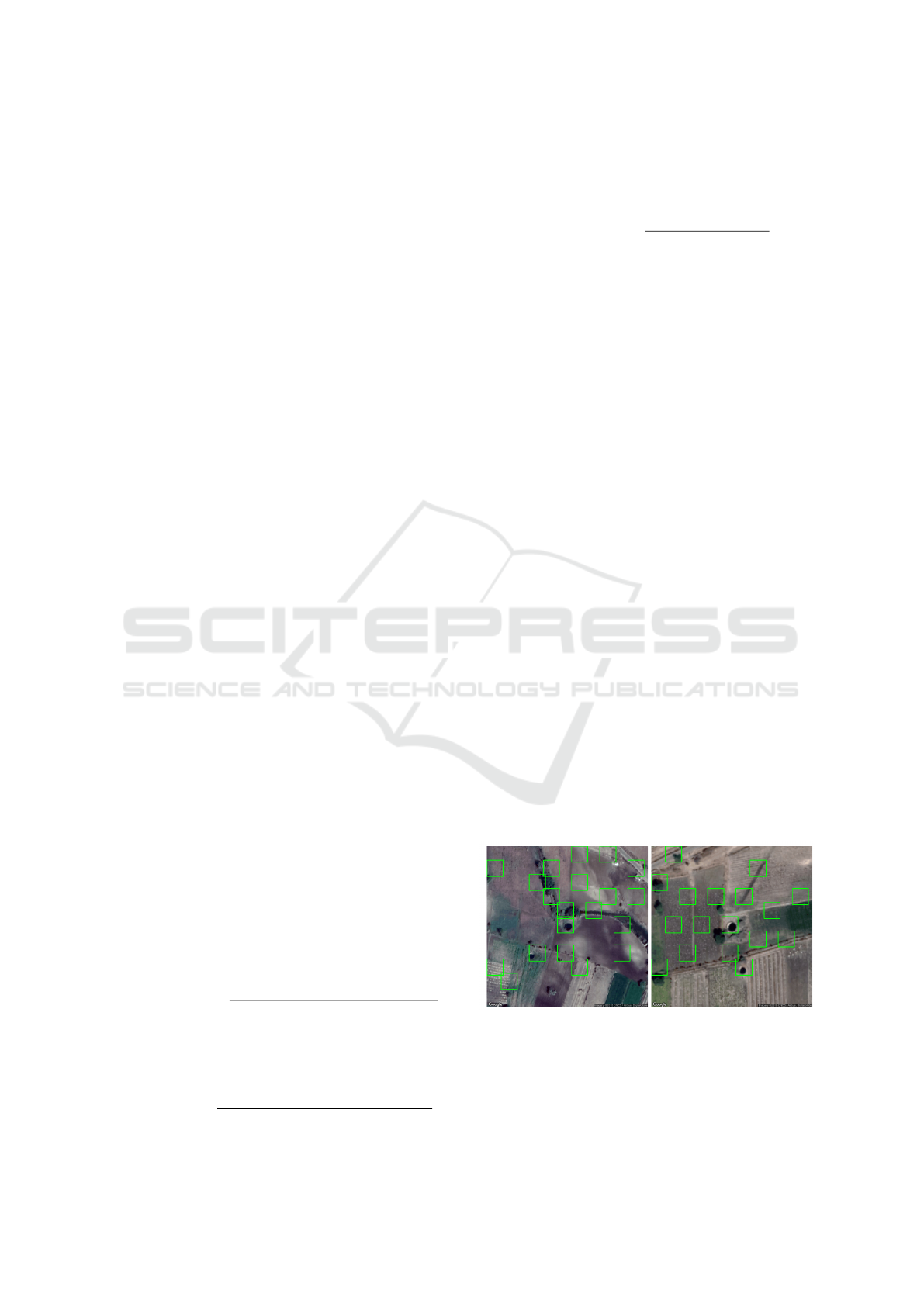
results are shown in figure 5.
Figure 5: Results of Basic CNN on 640 × 640 images.
• HaarCascade We trained using 1721 positive im-
ages and 3035 negative images and the results ob-
tained are shown in Figure 6. As can be seen
in Figure 6 the results obtained were terrible and
GISTAM 2019 - 5th International Conference on Geographical Information Systems Theory, Applications and Management
122
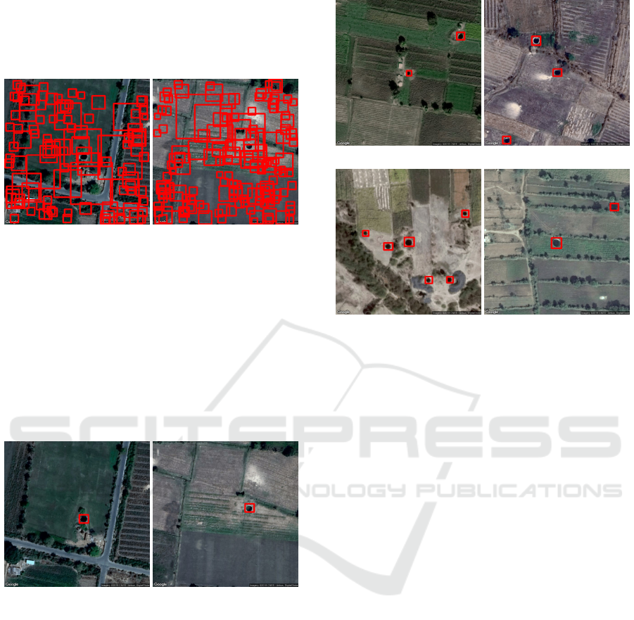
improving them will require a much larger num-
ber of positive and negative images which was not
feasible for us. Thus we dropped this algorithm
from comparison.
(a) (b)
Figure 6: (a) and (b) are results obtained from Haarcascade
method.
• HOG
We trained HOG using dlib on a machine which
has 8 GB RAM. The training was configured with
a learning rate of 0.01, epsilon value of 5 and slid-
ing window of 83 x 77 pixel.
The results obtained can be seen in Figure 7
which are promising thus we used this method for
comparison with other models.
(a) (b)
Figure 7: (a) and (b) are results obtained from HOG
method.
• YOLOv2
For training YOLOv2 and using it for detec-
tion we used darknet framework. The training
was performed on the standard configuration of
YOLOv2-VOC (yolov2-voc.cfg) it has a learning
rate of 0.001, the batch size of 64 and subdivisions
of 8. We used a weights file already pretrained
on Imagnet dataset (Russakovsky et al., 2015) and
trained on GPU (Nvidia Titan XP) for 20000 iter-
ations. The object detection was performed on the
default threshold value of 0.25 or more.
The results obtained are shown in Figure 8. This
result obtained is the best result achieved as com-
pared to methods which we discussed till now.
(a) Result-1 (b) Result-2
(c) Result-3 (d) Result-4
Figure 8: Results from YOLOv2 obtained from the weight
file trained for 20000 iterations.
• tinyYOLOv3
We used the Darknet framework for training and
detection. The training was performed on the
standard configuration of yolov3-tiny which is
a constrained network of YOLOv3 (yolov3-tiny-
obj.cfg) it has a learning rate of 0.001, the batch
size of 64 and subdivisions of 8 We used a weights
file already pretrained on Imagnet dataset (Rus-
sakovsky et al., 2015) and trained on GPU (Nvidia
Titan XP) for 20000 iterations. The object detec-
tion was performed on the default threshold value
of 0.25 or more. Similar results as YOLOv2 were
obtained for the images in Figure 8.
4.4 Retraining Surprise
One would think that inclusion of an image set in
training set will ensure that the trained model will give
high detection accuracy on that image set. However,
while this holds true for YOLO, surprising this is not
true for other object detection algorithms that we ex-
perimented with.
We validated the weights file obtained from train-
ing for 130 well images extracted randomly from any
district present in Maharashtra state for YOLO mod-
els. After validation, we found that in 100 images
from the validation dataset some of the wells present
were not getting detected thus we added those 100 im-
ages to the training dataset and retrained the network
for 20000 iterations. The results obtained before and
Well Detection in Satellite Images using Convolutional Neural Networks
123
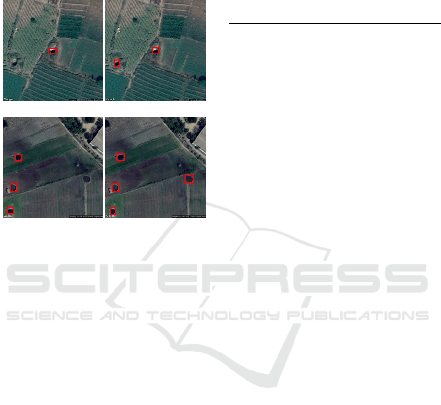
after retraining can be seen in Figure 9.
(a) (b)
(c) (d)
Figure 9: Figure (a), (c) are results obtained from YOLOv2
before validation and Figure (b), (d) are corresponding re-
sults after validation and retraining on YOLOv2.
The results show that if we retrain YOLO model
by including images in which wells were not getting
detected then the retrained model is able to detect the
similar wells which were not getting detected earlier.
This might be because the wells which were not get-
ting detected vary totally from the images for which
we have trained our model.
For the other object detection methods not based
on transfer learning, even after retraining the model
by including such images in training dataset, simi-
lar wells present in other images were not getting de-
tected. We have not been able to ascertain the reason
for the same.
4.5 Results
For testing we extracted 403 well images from 9 dis-
tricts of Maharashtra which includes Solapur, Kolha-
pur, Hingoli, Ratnagiri, Beed, Aurangabad, Chandra-
pur, Jalna, and Satara.
Then we tested the weights file of YOLOv2 and
tiny YOLOv3 obtained from 20000 iterations and
HOG using the svm file obtained after training on the
testing dataset.
The results can be seen in Table 1.
Thus the obtained precision and recall value on the
testing dataset for YOLOv2 is 0.95 and 0.91, for tiny
Table 1: Performance comparison of YOLOv2, tiny
YOLOv3 and HOG model.
Metric Model
Y OLOv2 tiny Y OLOv3 HOG
True Positive 592 529 226
False Positive 29 9 12
False Negative 58 100 430
Table 2: Precision-Recall trade-off between YOLOv2, tiny
YOLOv3 and HOG.
Model Precision Recall F1 Score
Y OLOv2 0.95 0.91 0.92
tiny Y OLOv3 0.98 0.84 0.90
HOG 0.95 0.34 0.51
YOLOv3 is 0.98 and 0.84 and for HOG is 0.95 and
0.34 respectively.
The precision-recall trade-off between these algo-
rithms is shown in Table 2. Based on these results, our
system uses YOLOv2 by default, but we provided the
option to user to chose tiny YOLOv3, HOG or other
algorithms if they wish.
5 CONCLUSIONS
We have built an open source system for well detec-
tion in satellite images and an associated annotation
system to annotate and validate identified objects in
satellite images. The advantage of the annotation sys-
tem is that we can use it to continuously grow our
dataset. We plan to use data augmentation technique
to create a larger dataset for transfer learning. Also,
YOLO was pre-trained on ImageNet (Russakovsky
et al., 2015) dataset which is very different from satel-
lite images. For the future work, we want to train
YOLO on some satellite image dataset, e.g, xView
dataset (Experimental, 2018). On top of that, we can
train it on our enhanced well dataset. Also, further
experimentation with several single shot object de-
tection algorithms has to be done along with transfer
learning to develop a robust system. Our aim would
be to generalize this satellite image object detection
procedure as much as possible to several classes of
objects.
REFERENCES
Albert, A., Kaur, J., and Gonzalez, M. C. (2017). Using
convolutional networks and satellite imagery to iden-
tify patterns in urban environments at a large scale.
CoRR, abs/1704.02965.
GISTAM 2019 - 5th International Conference on Geographical Information Systems Theory, Applications and Management
124

Chen, X., Xiang, S., Liu, C., and Pan, C. (2014). Vehicle
detection in satellite images by hybrid deep convolu-
tional neural networks. IEEE Geoscience and Remote
Sensing Letters, 11(10):1797–1801.
Cheng, M., Zhang, Z., Lin, W., and Torr, P. (2014). Bing:
Binarized normed gradients for objectness estimation
at 300fps. In 2014 IEEE Conference on Computer
Vision and Pattern Recognition, pages 3286–3293.
Dalal, N. and Triggs, B. (2005). Histograms of oriented gra-
dients for human detection. In 2005 IEEE Computer
Society Conference on Computer Vision and Pattern
Recognition (CVPR’05), volume 1, pages 886–893
vol. 1.
Experimental, D. I. U. (2018). Diux xview 2018 detection
challenge (http://xviewdataset.org).
LeCun, Y., Haffner, P., Bottou, L., and Bengio, Y. (1999).
Object recognition with gradient-based learning. In
Shape, Contour and Grouping in Computer Vision,
pages 319–, London, UK, UK. Springer-Verlag.
Maitra, M. K. (2011). Frequently asked questions
(faq) on groundwater - understanding the basics
(http://www.indiawaterportal.org/articles/frequently-
asked-questions-faq-groundwater-understanding-
basics).
Ministry of Water Resource, G. o. I. (2006a).
Census of minor irrigation schemes
(http://micensus.gov.in/censusmisch.html).
Ministry of Water Resource, G. o. I. (2006b).
Methodology of minor irrigation census
(http://micensus.gov.in/methodology.html).
Ministry of Water Resource, G. o. I. (2006c). National level
report - dugwell (http://micensus.gov.in/dugnat.html).
Qiu, S. (2017). Bbox-label-tool
(https://github.com/puzzledqs/bbox-label-tool).
Redmon, J., Divvala, S. K., Girshick, R. B., and Farhadi, A.
(2015). You only look once: Unified, real-time object
detection. CoRR, abs/1506.02640.
Redmon, J. and Farhadi, A. (2016). YOLO9000: better,
faster, stronger. CoRR, abs/1612.08242.
Redmon, J. and Farhadi, A. (2018). Yolov3: An incremental
improvement. CoRR, abs/1804.02767.
Ronacher, A. (2010). Flask (http://flask.pocoo.org/).
Russakovsky, O., Deng, J., Su, H., Krause, J., Satheesh, S.,
Ma, S., Huang, Z., Karpathy, A., Khosla, A., Bern-
stein, M., Berg, A. C., and Fei-Fei, L. (2015). Ima-
genet large scale visual recognition challenge. Int. J.
Comput. Vision, 115(3):211–252.
Vapnik, V. N. (1999). An overview of statistical learn-
ing theory. IEEE Transactions on Neural Networks,
10(5):988–999.
Viola, P. and Jones, M. (2001). Rapid object detection us-
ing a boosted cascade of simple features. In Proceed-
ings of the 2001 IEEE Computer Society Conference
on Computer Vision and Pattern Recognition. CVPR
2001, volume 1, pages I–I.
Wu, H., Zhang, H., Zhang, J., and Xu, F. (2015). Fast air-
craft detection in satellite images based on convolu-
tional neural networks. In 2015 IEEE International
Conference on Image Processing (ICIP), pages 4210–
4214.
Zhang, L., Shi, Z., and Wu, J. (2015). A hierarchical oil
tank detector with deep surrounding features for high-
resolution optical satellite imagery. IEEE Journal of
Selected Topics in Applied Earth Observations and
Remote Sensing, 8(10):4895–4909.
Well Detection in Satellite Images using Convolutional Neural Networks
125
