
Pattern-based Method for Anomaly Detection in Sensor Networks
Ines Ben Kraiem
1
, Faiza Ghozzi
2
, Andre Peninou
1
and Olivier Teste
1
1
Universit
´
e de Toulouse, UT2J, IRIT, Toulouse, France
2
Universit
´
e de Sfax, ISIMS, MIRACL, Sfax, Tunisia
Keywords:
Sensor Networks, Anomaly Detection, Pattern-based Method.
Abstract:
The detection of anomalies in real fluid distribution applications is a difficult task, especially, when we seek
to accurately detect different types of anomalies and possible sensor failures. Resolving this problem is in-
creasingly important in building management and supervision applications for analysis and supervision. In
this paper we introduce CoRP ”Composition of Remarkable Points” a configurable approach based on pattern
modelling, for the simultaneous detection of multiple anomalies. CoRP evaluates a set of patterns that are
defined by users, in order to tag the remarkable points using labels, then detects among them the anomalies
by composition of labels. By comparing with literature algorithms, our approach appears more robust and
accurate to detect all types of anomalies observed in real deployments. Our experiments are based on real
world data and data from the literature.
1 INTRODUCTION
Sensor networks play an important role in the super-
vision and exploration of fluid distribution networks
(energy, water, heating, . . . ) at campus or city scale.
The operation is based on the data collected by the
sensors. These data include anomalies that affect the
supervision (false alarms, billing errors,. . . ).
For instance, figure 1 illustrate a sudden change
(represented by a cross), in sensor measurements, that
generates a permanent level shift due to a hardware
problem (damaged sensors, sensor change, . . . ). The
triangles in the figure 1 includes several peaks repre-
senting reading defects related to an unforeseen event
(breakdown, break, . . . ). Finally, the rectangle rep-
resents a constant offset in the measurements due to
a communication problem between the supervision
devices. In this case, the sensor measurements may
differ from their expected values and thus become
anomalies making the exploration task more difficult
and complex. Therefore, all these scenarios must be
considered and must be accurately detected.
In this context, anomaly detection appears to iden-
tify and to find values in data that do not conform to
expected behavior (Chandola et al., 2009). Beyond
the supervision of sensor networks, there is a wide
range of applications for which it is essential to de-
tect anomalies to facilitate data analysis including in-
trusion detection, industrial damage detection, image
processing and medical anomaly detection, textual
anomaly detection, habitat monitoring, online trans-
actions and fraud detection etc ((Hodge and Austin,
2004), (Agrawal and Agrawal, 2015)). Several tech-
niques have been proposed in the literature and cat-
egorized according to the fields of application or the
types of anomalies to be detected (Chandola et al.,
2009). Nevertheless, these techniques are unable to
always detect all types of anomalies simultaneously
and thus real applications are forced to use several
methods to accurately detect all existing anomalies.
This paper is placed in the context of real applications
with anomalies specific to the business (fluid manage-
ment on the Rangueil-Toulouse campus). The prob-
lem is to find a method to detect multiple anomalies
of different types (special event, sensor malfunctions)
observed during actual deployments while maximiz-
ing the number of anomalies detected and minimizing
errors. In this context, we deal with univariate time
series.
The difficulty of having a robust technique to de-
tect all the anomalies leads us to define a new con-
figurable method named CoRP ”Composition of re-
markable points”. This method allows, firstly, to de-
tect points that appear remarkable in the time series
by evaluating patterns and, secondly, to create re-
markable point compositions used to identify multiple
anomalies.
The remainder of this paper is structured as fol-
lows. In section 2, we provide some techniques and
algorithms mentioned in the literature about anomaly
104
Ben Kraiem, I., Ghozzi, F., Peninou, A. and Teste, O.
Pattern-based Method for Anomaly Detection in Sensor Networks.
DOI: 10.5220/0007736701040113
In Proceedings of the 21st International Conference on Enterprise Information Systems (ICEIS 2019), pages 104-113
ISBN: 978-989-758-372-8
Copyright
c
2019 by SCITEPRESS – Science and Technology Publications, Lda. All rights reserved

Figure 1: Example of defects in sensor measurements.
detection in time series. Then, in section 3, we de-
scribe our pattern-based method for anomaly detec-
tion. In section 4, we detail the experimental setup,
the case study with the real world data sets and a
benchmark data sets. In section 5 we conclude with
the perspectives and ideas for further research.
2 STATE OF THE ART
Existing Surveys on Anomaly Detection. Most of
the existing research relates to either several applica-
tion domains or a single field of application, as in the
case of these reviews ((Chandola et al., 2009), (Hodge
and Austin, 2004), (Sreevidya et al., 2014), (Agrawal
and Agrawal, 2015)). Among these applications we
can mention, intrusion detection, industrial damage
detection, image processing and medical anomaly de-
tection, textual anomaly detection, habitat monitor-
ing, online transactions and fraud detection. The au-
thors discussed several anomaly detection techniques
according to the field of application. Typical exam-
ples include approaches based on clustering, classifi-
cation, statistics, nearest neighbors, regression, spec-
tral decomposition, and information theory. These
techniques can detect three types of anomaly: point,
contextual and collective anomalies.
Anomaly Detection on Time Series. Some authors
have chosen techniques that are appropriate for de-
tecting particular types of anomalies observed in real
deployments (Sharma et al., 2010). Thus, these au-
thors have explored anomaly detection techniques
that are appropriate for detecting anomaly types
(short, noise, and constant faults). They explore four
qualitatively different classes of fault detection meth-
ods namely: rule-based methods (short, noise, con-
stant rules), least-squares estimation-based method,
learning-based methods (HMM) and Time-series-
analysis-based methods (ARIMA). Although each of
these methods detects specific types of anomalies,
they still generate errors, especially in a context of
multiple anomalies. For this reason, the authors used
hybrid methods, Hybrid(U) and Hybrid(I), to improve
their results and reduce respectively the number of
false negative and false positive. Hybrid(U) declares a
point as an anomaly if at least one of the methods ex-
plored identified that point as an anomaly, while Hy-
brid(I) declares a point as an anomaly when all the
explored methods identified this point as an anomaly.
(Yao et al., 2010) propose an approach to on-
line anomaly detection in measurements collected by
sensor systems. They propose an algorithm termed
Segmented Sequence Analysis (SSA) that consists on
comparing the collected measurements against a ref-
erence time series. SSA leverages temporal and spa-
tial correlations in sensor measurements. This method
also fails to accurately detect all anomalies. Thus,
the authors proposed an hybrid approach to improve
the results. Typically, a combination of SSA with the
rule-based method (short and constant rules). Indeed,
they start by applying the rule-based method to detect
short-term anomalies, then they apply SSA to detect
the remaining anomalies.
Other methods for anomaly detection in an uni-
variate data-set are using an approximately normal
distribution of data such that generalized ESD test
(Extreme Studentized Deviate) (Rosner, 1983) and
Change Point (Basseville et al., 1993) (Aminikhang-
hahi and Cook, 2017). The limitation of ESD is that it
requires to specify an upper bound for the suspected
number of outliers. This is not possible on all ap-
plications and is impossible for online anomaly de-
tection. Change Point detects distribution changes
(e.g., mean, variance, covariances) in sensor mea-
surements. This method detects each change as an
anomaly meanwhile changes may exist in the time se-
ries that do not necessarily represent an anomaly and
vice versa.
Other methods are based on the nearest neighbor
anomaly detection technique and can be grouped into
two categories (Chandola et al., 2009): (1) techniques
that use the distance of a data instance to its kth near-
est neighbor as the anomaly score (Upadhyaya and
Singh, 2012). (2) techniques that compute the relative
density of each data instance to compute its anomaly
score for example LOF (Local Outlier Factor) algo-
rithm (Breunig et al., 2000). One of the drawbacks of
Nearest Neighbor Based Techniques is, that it fails to
label data correctly if the data has normal instances
that do not have enough close neighbors or if the
data has anomalies that have enough close neighbors
(Chandola et al., 2009).
While each of these methods has been designed
for anomaly detection, we believe that they do not
satisfy all the desirable properties described above
Pattern-based Method for Anomaly Detection in Sensor Networks
105

including the detection of all types of anomalies si-
multaneously observed in actual deployments with
the less error possible. Additionally, several methods
among the mentioned methods require pre-treatment
or post-treatment with hybrid methods to improve
their results. To evaluate the performance of these
methods, we have selected algorithms that belong to
different techniques and are close to detect the types
of anomalies we seek to detect.
We will present these algorithms in the following
paragraph and illustrate a comparison between these
methods on our case study in the section 4.
Exploration of Existing Detection Methods. In
our study, we explored five methods that belong to
four different techniques to detect the types of anoma-
lies observed in our application.
• The rule-based methods that belong to the classi-
fication technique and that can be extremely pre-
cise, but their accuracy depends essentially on
the choice of parameters; This method is based
on the exploitation of domain knowledge to de-
velop heuristics to detect and identify sensor de-
fects (Sharma et al., 2010). In our exploration, we
used two rules to detect short (abnormal change)
and constant anomalies (no variation):
Short Rule: We process the time series by com-
paring two successive observations each time. An
anomaly is detected if the difference between
them is greater than a threshold. To automatically
determine the threshold, we used the histogram-
based approach (Ramanathan et al., 2006). We
have plotted the histogram of the sensor reading
change between two successive samples for the
short rule and then select one of the histogram
modes as a threshold.
Constant Rule: We calculate the standard devia-
tion for a set of successive observations. If this
value is equal to zero, the set is declared as an
anomaly.
• Density-based method that consists in comparing
the density around a point with respect to the den-
sity of its local neighbors. It can detect local and
global anomalies (abnormal change). (Breunig
et al., 2000) proposed the LOF algorithm. In this
method, the anomaly scores are measured using
a local outlier factor, which is the ratio of the lo-
cal density around this point to the local density
around its nearest neighbor. The data point whose
LOF value is high is declared anomaly. The effec-
tiveness of LOF is strongly depends on the choice
of the number of closest neighbors.
• Statistics-based method: First, we used ESD
method for the automatic detection of anoma-
lies and more precisely the abnormal change such
as positive or negative peaks. Secondly, we
used the point change method to detect the level
shift. AnomalyDetection is an open source R
package for detecting anomalies in the presence
of seasonality and an underlying trend. This
package is based on the SH-ESD (Seasonal Hy-
brid ESD) algorithm, developed by (Hochenbaum
et al., 2017), which first uses the STL time series
decomposition (Seasonal and Trend decomposi-
tion using Loess) developed by (Cleveland et al.,
1990) to divide the time series signal into three
parts: seasonal, trend and residue. Secondly, it ap-
plies residual anomaly detection techniques such
as ESD (Rosner, 1983) using statistical metrics.
For point change detection, this is the name given
to the problem of estimating the point at which
the statistical properties of a sequence of observa-
tions change (Aminikhanghahi and Cook, 2017).
We used the ChangePoint package, in R, which
implements various point change methods in the
(single and multiple) data to detect either mean or
variance breaks or breaks in both the average and
in the variance. ESD and point change is consid-
ered light. statistical techniques in terms of calcu-
lation.
• Method based on time series analysis: The prin-
ciple of this approach is to use temporal correla-
tions to model and predict time series values. In
this article, we used the ARIMA model (AutoRe-
gressive Intergrated Moving Average) to create a
prediction model according to the approach de-
scribed by (Chen and Liu, 1993). ARIMA is ef-
ficient in anomaly detection with seasonal data.
Thus, this method can detect different types of
anomalies such as Additive Outlier (AO), Inno-
vation Outlier (IO), Level Shift (LS), Temporary
change (TC) and Seasonal Additive Outlier (SA).
What interests us among these types are Additive
Outlier (AO) which represent in our case an ab-
normal change and Level Shift (LS) and Tempo-
rary change (TC).
There are open source implementations for algo-
rithms like LOF, ARIMA, S-H-ESD and Change
Point and we have implemented other approaches
(Short rule and Constant rule) depending on available
sources.
Table 1 represents a summary of the methods we
have explored to detect defects found in actual de-
ployments and presented in figure 1. So, we used
Short rule, ARIMA, LOF and S-H-ESD algorithms to
detect positive and negative peak. Then, we explored
Constant rule to detect constant anomalies and finally
ICEIS 2019 - 21st International Conference on Enterprise Information Systems
106

Table 1: Positioning detection methods against anomalies to be detected.
Type of anomalies Detection methods
Positive and Negative peak Short Rule, ARIMA, LOF, S-H-ESD
Constant Constant Rule
Level Shift ARIMA, Change Point
we used ARIMA and Change Point to detect Level
Shift also known in literature by Concept Drift. In
this paper we will remain on the terminology of Level
Shift.
3 METHODOLOGY
Several anomalies have been observed by the ana-
lysts in real deployments and they occur as a result
of communication problems between supervision de-
vices, failures, stops of sensors or changes of sen-
sors. Sensor networks are monitored by the experts,
by observing the curves, in order to detect points that
seem remarkable and that illustrate unusual behaviors
in the real context. These remarkable points are un-
usual variations between successive points of a time
series and which are the markers (or indices) of pos-
sible anomalies. In this context, we have created our
configurable approach, called CoRP (”Composition
of Remarkable Points”). It is based on patterns to
detect remarkable points and on compositions of re-
markable points to identify anomalies.
3.1 Notations
Definition 1. A time series is composed of successive
observations or points collected sequentially in time
at a regular interval. These observations represent the
measures that are associated with a timestamp indi-
cating the time of its collection.
Let Y
i
=
{
y
1
, y
2
, y
3
....
}
be a time series represent-
ing the sequence of collected sensor measurements y
i
∈ R for each observation i ∈ N.
Definition 2. A point is a measure composed of a
value and a time stamp. In this paper, we note a mea-
sure y
j
= (t
j
, v
j
) such as t
j
is the timestamp of y
j
(called t(y
j
)) and v
j
is the value of y
j
(called v(y
j
)).
3.2 Description of CoRP Method
Based on the experience of experts (detection of re-
markable points and identification of anomalies), the
CoRP algorithm is built in two phases. The first one
is dedicated to detect the points considered as remark-
able in the time series. The second phase is dedi-
cated to identify anomalies by using compositions of
remarkable points.
3.2.1 Detection of Remarkable Points
The detection of remarkable points is made from the
detection patterns.
Definition 3. A pattern is defined by a triple (l, σ
a
,
σ
b
) where l is a label that characterizes the pattern.
σ
a
and σ
b
are two thresholds used to decide if a point
is remarkable (or not). A pattern is applied to three
successive points of a time series. We denote three
successive points y
j−1
, y
j
, y
j+1
of a time series Y as
y
minus
, y, y
plus
. σ
a
is the difference between v(y
minus
)
and v(y) whereas σ
b
is the difference between v(y)
and v(y
plus
) as shown in the figure 2 . When a pattern
is checked on y
minus
, y, y
plus
, the label l of the pattern
is used to label the point y.
Figure 2: Example of pattern.
Definition 4. A labeled time series is a time series of
points on which the labels detected by the patterns are
added.
Definition 5. A point y
i
of a labeled time series is
defined by a triple (t
i
, v
i
, L
i
) where t
i
is the timestamp,
v
i
is the value and L
i
=
{
l
1
, l
2
, ...
}
is a list of labels that
characterizes the point as a remarkable point.
So, the patterns are independently used to detect
remarkable points and add them their corresponding
label. Thus, the list of labels of a point consists of all
the labels of all the different patterns that are triggered
on this point. The figure 3 illustrates an extract from a
labeled time series of index data that tends to grow. It
presents four examples of patterns (Normal, Ptpicpos,
Ptpicneg, Changniv). Let us notice the point number
4 which includes two labels (Ptpicneg, Changniv).
Pattern-based Method for Anomaly Detection in Sensor Networks
107

Figure 3: Labellization of a remarkable point ”y” by a pat-
tern.
Example. Let us give some examples of patterns de-
fined with the help of the experts and used to label the
curve of the figure 3 :
• remarkable ”Positive Peak Point” (Ptpicpos, 100,
100) where Ptpicpos represents the descriptive la-
bel of the pattern, σ
a
= 100 and σ
b
= 100;
• remarkable ”Negative Peak Point” (Ptpicneg, -
100, -100);
• remarkable ”Level Shift” (Changniv, -1000, -
100).
The Algorithm 1, called EvaluatePattern, allows
to evaluate the patterns using rules. This function
takes as input three successive points denoted y
minus
,
y and y
plus
and the pattern to be evaluated, and returns
the result of the evaluation: the pattern is triggered
or not. Different verification rules are applied by the
algorithm according to the signs of σ
a
and σ
b
. The
rules to compare y
minus
and y according to σ
a
are:
• If σ
a
> 0, the rule is v(y) >= v(y
minus
) + σ
a
;
• If σ
a
< 0, the rule is v(y) <= v(y
minus
) + σ
a
;
• If σ
a
= 0, the rule is v(y) = v(y
minus
);
The rules to compare y and y
plus
according to σ
b
are
similar (see Algorithm 1).
Algorithm 2 uses the EvaluatePattern function to
process a time series. It takes as input the initial time
series and the list of patterns and returns a new labeled
time series. The processing consists in browsing the
time series and, for each pattern, add the label pattern
to the point when the pattern is triggered.
The result of Algorithm 2 is a labeled time se-
ries (points tagged with labels). The figure 4 presents
an example of labeled time series produced by Algo-
rithm 2. Just notice that a point can be labeled with
one or more labels.
Figure 4: Labelization of a series by remarkable points.
Algorithm 1: Pattern evaluation.
function BOOLEAN EVALUATEPAT-
TERN(y
minus
, y, y
plus
, p)
Input y
minus
, y, y
plus
: point, p=(L
p
, σ
a
, σ
b
): pattern
Output Boolean
if p.σ
a
> 0 then
left←(v(y) ≥ v(y
minus
) + p.σ
a
? true:false)
else if p.σ
a
< 0 then
left←(v(y) ≤ v(y
minus
) + p.σ
a
? true:false)
else if p.σ
a
= 0 then
left←(v(y) = v(y
minus
)? true:false)
end if
if p.σ
b
> 0 then
right←(v(y) ≥ v(y
plus
) + p.σ
b
?true:false)
else if p.σ
b
< 0 then
right←(v(y) ≤ v(y
plus
) + p.σ
b
? true:false)
else if p.σ
b
= 0 then
left←( v(y) = v(y
plus
)? true:false)
end if
return (left and right)
end function
3.2.2 Composition of Patterns
Experts can find anomalies by searching for spe-
cific combinations of remarkable points and by com-
paring their corresponding values. So, the goal is
to model these particular successions of remarkable
points. From a subset of points of a labeled time se-
ries, we can construct a composition of labels by con-
catenation of the L
i
labels of these remarkable points.
Such compositions of labels are used to detect anoma-
lies. Finally, an anomaly is recognized by a compo-
sition of labels on successive points and the verifica-
tion of conditions on the values of the corresponding
points.
Definition 6. An anomaly can be find starting from a
remarkable point from which are checked i) a compo-
sition of labels in the following points and ii) a condi-
tion expressed on the values of the points involved in
ICEIS 2019 - 21st International Conference on Enterprise Information Systems
108

Algorithm 2: Remarkable point detection.
Input Y =
{
y
1
, y
2
, y
3
....
}
: time series,
P =
{
p
1
, p
2
, p
3
....
}
: list of patterns
Output Y
L
a labeled time series
for i in range(2..|Y |-1) do
for k in range(1..|P|) do
if EvaluatePattern(y
i−1
,y
i
,y
i+1
,p
k
) then
L
i
< −L
i
+ p
k
.L // Add p
k
.L to y
i
labels
end if
end for
end for
return Y
L
the composition. The anomaly is finally identified on
one or more points of this composition.
Figure 5: Grammar for the definition of a composition of
labels.
To define a composition of labeled points, we pro-
pose a grammar, illustrated in the figure 5, which de-
fines the elements of a composition of labels. The
grammar is expected to define the possible labels (one
or more) on successive points that allow to recognize
a composition of labels. The grammar starts from la-
bels placed on the points (<label>). Labels can be
combined on a single point with logical expressions
AND, OR and NOT . For example, ”l1 AND NOT l2
AND l3” designates a point labeled with l1, labeled
with l3 and not labeled with l2. Each label compo-
sition on a single point can be repeated on successive
points by quantifiers: ?, + and * (<label-enum>). For
example, ”(l1)+” then means one or more successive
points labeled with l1. The final label composition
is defined by successive combinations of different la-
bels on single or multiple points by using ”.” opera-
tor (<composition>). For example, ”l1.(l2)*.l1 OR
l3” means a point labeled with l1 followed by zero or
more points all labeled with l2 followed by a point
labelled with l1 or with l3.
Definition 7. Composition of labels Thus, a compo-
sition of labels to recognize an anomaly is composed
of three parts:
• composition: the composition of the labels on
successive points. It is defined according to the
grammar presented in the figure 5;
• condition: a condition between the values of the
recognized points corresponding to the sequence
of the labels of the composition. Indeed, the same
label composition on successive points can cor-
respond to different anomalies and the condition
allows to identify only one anomaly. This con-
dition on values is a classical condition created
using the operators (<, <=, ...) to compare val-
ues and logical operators (and/or/not) to combine
comparisons. To avoid the use of v(y) notation,
we denote by v
i
the value of the ith point recog-
nized by the composition, v
1
the first one and v
n
the last one; note that the number of points in-
volved in the composition can be variable;
• conclusion: the identified anomaly for which are
indicated its type (name of the anomaly) and the
list of points where the anomaly is.
We can thus define label compositions to identify
anomalies. For example, we give hereafter three ex-
amples of anomalies to be detected as presented in
the introduction: i) anomaly of constant values, ii)
anomaly of values in negative peak, iii) anomaly of
values in positive peak; the latter is possibly recog-
nized from 2 label compositions.
Some composition of labels to recognize the
above anomalies are given hereafter:
Label-composition 1
composition: Begincstpos . Cst* . Endcstneg;
condition: v
1
== v
2
and v
n−1
== v
n
;
conclusion: constant − > all;
Label-composition 2
composition: Normal . Ptpicpos . Ptpicneg . Normal;
condition: v
2
< v
4
and v
3
< v
1
;
conclusion: negative peak − > v
3
;
Label-composition 3
composition : Normal . Ptpicpos . Ptpicneg . Normal;
condition: v
2
> v
4
and v
3
> v
1
;
conclusion: positive peak − > v
2
;
Label-composition 4
composition: Normal . Ptpicpos . Ptpicneg AND
Changnivneg . Normal;
condition: v
2
> v
n
and v
n−1
> v
1
;
conclusion : positive peak − > v
2
;
Let us consider the compositions presented in the
figure 4 in red. The indices ranging from 2 to 5 give
the following series of labels: ( Normal . Ptpicpos .
Ptpicneg and Changnivneg . Normal) detected by the
composition of labels 4 of the examples above. This
composition makes it possible to detect the positive
peak anomaly in 3 when considering the condition.
Pattern-based Method for Anomaly Detection in Sensor Networks
109

The index points from 8 to 11 (”Normal . Ptpic-
pos . Ptpicneg . Normal”) , triggers the label compo-
sitions 3 and 2:
• Label composition 3: the condition leads to v
9
>
v
11
and v
10
> v
8
which is false so the composition
is not valid;
• Label composition 2: the condition leads to v
9
<
v
11
and v
10
< v
8
which is true therefore the com-
position is valid and the Negative Pic anomaly is
recognized in point 10 (v
10
);
4 EXPERIMENTAL SETUP
In this section, we will first introduce our case study.
Then we analyze the results of the algorithm of the
literature as well as our algorithm on our data sets.
Then, we evaluate more these algorithms with bench-
marks data and finally, we present the computational
performances of the algorithms explored.
4.1 Description of the Case Study
The field of application treated in this paper, is the
sensor network of the Management and Exploitation
Service (SGE) of Rangueil campus attached to the
Rectorate of Toulouse. This service exploits and
maintains the distribution network from the data re-
lated to the different installations. More than 600 sen-
sors of different types of fluids (calorie, water, com-
pressed air, electricity and gas), which are scattered in
several buildings, are managed by the SGE supervi-
sion systems. For this paper, we focus on calorie data
and we processed 25 sensors. Thus, we analyze calo-
rie measurements collected every day for more than
three years collected from the 25 sensors deployed
in different buildings: 1453 data per sensor which is
36325 data points in total. The measurements of these
sensors are reassembled at a regular frequency and
represent the indexes (readings of sensors) which are
used to measure the quantities of energy consumed
(by successive value differences, consumption). We
were able to identify the types of anomalies that ex-
ist in the calorie data through the knowledge gained
from the SGE experts by visually inspecting the data
sets. The examples of faults presented in the figure
1 are taken from these same data sets. The predomi-
nant anomaly in these readings is the constant values,
nearly 8578 observations on all the data and this is
following the stopping of the sensors. We also found
among these values, several constants with an offset.
Typically, a constant with a level shift that begins with
a positive or negative peak. Then, there is a lot of
abnormal change such as positive or negative peaks,
nearly 380. And finally, there is eight level shift due
to sensor change. In order to detect the remarkable
points, we created 14 patterns and 12 label compo-
sitions of these patterns to detect the anomalies de-
scribed above.
4.2 Experimentation on Real Case Time
Series
In this part, we explore the different anomaly detec-
tion methods described in Table 1. Our motivation
to consider these methods is to broaden the scope
of analysis to test their effectiveness in detecting the
anomalies considered in this paper and to compare the
results against our approach. As noted above, these
techniques have proven effective in detecting anoma-
lies in the sensor data. On the other hand, as we
will see through the results of the experiments, none
of these methods is perfect to detect all the types of
anomalies that we observed in the real deployments.
Thus, we present an evaluation of the following meth-
ods: Short rule, Constant rule, LOF, ARIMA, S-H-
ESD and the change of point. We applied these meth-
ods by category of anomalies as indicated in the Ta-
ble 1. In order to evaluate the performance of these
methods we use the number of true positives (true
detected anomalies ), the number of false positives
(false detected anomalies ) and the number of false
negatives (true undetected anomalies) as evaluation
metrics. The results are presented in the figure 6 as
follows: the method based on the Short rule and the
method based on the Constant rule are noted SR and
CR respectively while the Change Point is noted LS.
For each method we also report the Precision, Re-
call, F-measure metrics to compare and evaluate the
results of anomaly detection. As shown in Figure 6A
and B, we applied methods that are able to detect the
abrupt change between two successive samples that
could be a positive or negative peak or a small vari-
ation. We presented LOF results in a separate chart
Table 2: Evaluation of anomaly detection methods for index
data sets.
Evaluation Precision Recall F-
measure
SR 0.52 0.17 0.32
CR 1 0.80 0.88
LOF 0.022 0.12 0.022
S-H-ESD 0.34 0.40 0.36
ARIMA 0.30 0.07 0.11
LS 0.29 0.87 0.43
CoRP 1 1 1
ICEIS 2019 - 21st International Conference on Enterprise Information Systems
110
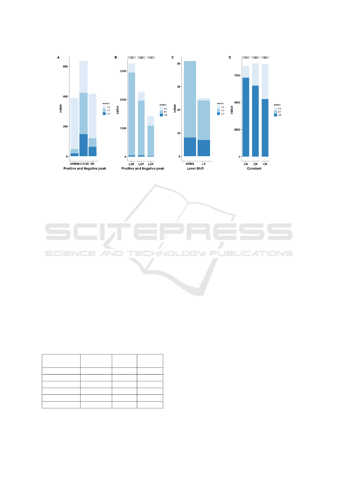
Figure 6: Evaluation of anomaly detection methods on index data.
for more visibility. These methods are not fully auto-
mated and therefore we need to select the parameters
such as the threshold for the short rule, the neighbor
number for LOF or the model type for ARIMA etc.
The LOF method, which is based on the nearest K
neighbors, produces an index, called the score func-
tion, which represents the degree of anomaly assumed
for the observations. It is then sufficient to define a
threshold to qualify the ”normal” and ”abnormal” re-
sults. In our experiments we have varied the choice
of K in a range of 30 to 10 in order to evaluate the
influence of this parameter on the detection result and
we have judged a threshold = 1.5 corresponding to an
observation in the standard of distribution scores. For
the Short rule, we need to set a threshold to compare
it with the variation between successive observations.
To this end, we used the histogram-based method de-
scribed in Section 5.2. And finally, for the Constant
rule, we have varied the choice of size of sliding win-
dow in a range of 30 to 10.
Based on the results presented in the Figure 6, we
make the following observations: LOF is the method
Table 3: Evaluation of anomaly detection methods in con-
sumption data sets.
Evaluation Precision Recall F-
measure
SR 0.66 0.63 0.64
CR 1 0.72 0.83
LOF 0.39 0.78 0.52
S-H-ESD 0.41 0.80 0.54
ARIMA 0.66 0.25 0.36
CoRP 1 0.98 0.98
that generates the most false positives while ARIMA
generated the most false negatives. The S-H-ESD
method is the method that can detect the most True
positive among them, but on the other hand it causes
a lot of false positives and false negatives. Then the
method based on the Short rule detects fewer anoma-
lies by comparing with S-H-ESD. However, it causes
fewer false positives than the other methods.
Based on Table 2 and figure 6 we observe that: i)
the efficiency of the Constant rule or the LOF method
strongly depends on the choice of the sliding window
or the number of neighbors. ii) The Change Point
method works well when there is actually a true level
shift in the time series but however, in the absence
of anomaly it has a low accuracy. iii) Between the
Short rule, ARIMA and S-H-ESD, the Short rule is
the most accurate and ARIMA is the least efficient for
detecting abnormal change. By comparing with these
methods, our CoRP algorithm can detect all types of
anomalies with better accuracy and recall. In effect,
CoRP works very well on the index data and typically
on our real case study.
To further evaluate our algorithm and to demon-
strate the effectiveness of the anomaly detection
methods, we used SGE consumption data. So, we
took the measurements that come from 25 sensors.
Consumption data are seasonal data and their daily
evolution, unlike index data, are somewhat variable.
We have manually inspected these data to understand
how these data work and to create patterns of anoma-
lies that may exist. The anomalies we have seen in
the data are: positive and negative peaks, constant
anomalies, constants that start and end with a big
peak. Since the data is not stationary, we did not ap-
Pattern-based Method for Anomaly Detection in Sensor Networks
111

Table 4: Evaluation of anomaly detection methods in Benchmark data sets.
Datasets HIPC IPI
Algorithm
Evaluation
Precision Recall Precision Recall
CoRP 1 0.80 0.75 0.75
ARIMA 1 1 1 1
LOF 0.11 0.20 0 0
S-H-ESD 0.20 0.20 0.33 0.25
RC 0 0 0 0
LS 0 0 0 0
ply the Change Point algorithm because there is no
level shift in this data to be detected. Thus we have
created 9 patterns to detect remarkable points and 5
label compositions to detect anomalies.
According to the results presented in figure 6, we
can say that the number of neighbors equal to 20 is the
most appropriate choice to detect the most anomalies
in LOF algorithm. However, for the Constant rule,
it is important to use a window size small enough to
handle data sets containing a large number of con-
stant values. It can be seen from Table 3 that the
literature algorithms are much more efficient on the
consumption data by comparing with the index data.
Even with this type of data, our approach has obtained
the best result of F-measure by comparing with other
algorithms. Actually, he detected the most anomalies
with the least possible errors with a precision equal to
1 and a recall equal to 0.98. Then, the result of the
rule-based method (SR, CR) and the ARIMA method
was close to the best and obtained the best accuracy
with respect to LOF and SH-ESD. On the other hand,
SH-ESD is the method that was closest to the best
result in terms of recall with a value equal to 0.80.
But it should be noted, that these algorithms that we
evaluated cannot detect all the types of anomalies ob-
served in the data which means that each algorithm
is efficient in a specific type. The particularity of our
method is that we can set the patterns and the compo-
sition of labels according to our needs to detect, with a
great precision and efficiency, all the types of anoma-
lies observed in the real deployments.
4.3 Experimentation on Benchmark
Data Set
In order to evaluate the algorithm in another con-
text, different to our case study, we used the data sets
used in the package developed in R and implements
ARIMA method (L
´
opez-de Lacalle, 2016). Among
this data, we explored the data of HIPC (Harmonised
Indices of Consumer Prices). This data sets repre-
sent Harmonised indices of consumer prices in the
Euro area. Also, we explored the data of IPI (Indus-
trial Production Indices ). It represents the industrial
production indices in the manufacturing sector of Eu-
ropean Monetary Union countries(L
´
opez-de Lacalle,
2016). Each of these data sets contains several time
series which present monthly data from 1995 to 2013.
We tested two time series of these two data sets. Each
of them contains 229 measurements with 5 anoma-
lies in HIPC and 4 anomalies in IPI. These anomalies
are a mix of AO (Additive Outlier), TC (Temporary
Change) or LS (Level Shift).
Thus, we analyzed the characteristics of these data
and the curve that represents the time series to be able
to specify the patterns. So, we first created a different
patterns to detect the remarkable points in the time
series. Then we made a composition of these patterns
to detect anomalies.
Table 4 is a comparison between the literature al-
gorithms and our algorithm, on the data used in the
ARIMA package. We did not test the constant rule in
the HIPC and IPI datasets because the anomalies ob-
served in these data do not contain a constant anoma-
lies. Therefore, we applied CoRP, ARIMA, LOF with
a number of neighbors equal to 20, S-H-ESD, Change
Point and the Short rule on these data. The algorithm
based on the Short rule and Change Point are the
worst among these algorithms, while our algorithm
is the best among them and can detect the majority of
anomalies observed with few errors.
4.4 Complexity
In this part, we focus on the computing time required
by the different methods of literature and our algo-
rithm. The experiments are performed on machine
running windows 10 professional and optimized by an
Intel (R) Core (TM) i5 processor and 16GB of RAM.
We used the Python 3.7 Anaconda open source dis-
tribution to turn our algorithm and R 3.5 to turn the
algorithms of the literature. We calculated the execu-
tion time of index data for each algorithm we evalu-
ated to compare it with the execution time of our algo-
ICEIS 2019 - 21st International Conference on Enterprise Information Systems
112

rithm. The algorithms according to their run-time per-
formance are as follows: The rule-based method and
the S-H-ESD method are the fastest with an execution
time of 0.5s. Then, the LOF method with an execu-
tion time equal to 2.5s. Subsequently our algorithm
with 5.40s of execution time and finally ARIMA with
7.60s.
5 CONCLUSION
Anomaly detection in supervisory applications is very
important especially in the field of sensor networks.
This paper represents the CoRP approach based on
patterns applied to the univariate time series of sen-
sor data. This method is very effective at simultane-
ously detecting different types of anomalies observed
during actual deployments. Our algorithm is com-
posed of two steps: it marks (labels) all the remark-
able points present in the time series on the basis of
patterns of detection. Then, he precisely identifies
the multiple anomalies present by label compositions.
This approach requires application domain expertise
to be able to efficiently define patterns. Our case
study is based on a real context: sensor data from the
SGE (Rangueil campus management and operation
service in Toulouse). The evaluation of this method
is illustrated by first using the index and consumption
data of calorie sensors operated by the SGE and, sec-
ondly, by using datasets from the scientific literature.
We compare our algorithm to five methods belong-
ing to different anomaly detection techniques. Based
on the precision, recall, f-measure, evaluation crite-
ria, we show that our algorithm is the most efficient
at detecting different types of anomalies by minimiz-
ing false detections. There are several extensions of
this research, among them: i) Use learning methods to
automate the algorithm, model the patterns automati-
cally and improve its performance in terms of calcu-
lation ii) Apply our algorithm on data streams, which
are generated continuously, to trace alarms as early
as possible and detect anomalies even before storing
them in the databases.
ACKNOWLEDGEMENT
This work is in collaboration with the the Manage-
ment and Exploitation Service (SGE) of Rangueil
campus attached to the Rectorate of Toulouse. The
authors would like to thank the SGE, directed by Vir-
ginie Cellier, to provide us with access to sensor data
from their databases. Also, they are grateful for the
experts who have facilitated the understanding of the
data and anomalies observed in actual deployments.
REFERENCES
Agrawal, S. and Agrawal, J. (2015). Survey on anomaly de-
tection using data mining techniques. Procedia Com-
puter Science, 60:708–713.
Aminikhanghahi, S. and Cook, D. J. (2017). A survey
of methods for time series change point detection.
Knowledge and information systems, 51(2):339–367.
Basseville, M., Nikiforov, I. V., et al. (1993). Detection of
abrupt changes: theory and application, volume 104.
Prentice Hall Englewood Cliffs.
Breunig, M. M., Kriegel, H.-P., Ng, R. T., and Sander, J.
(2000). Lof: identifying density-based local outliers.
volume 29, pages 93–104. ACM sigmod record.
Chandola, V., Banerjee, A., and Kumar, V. (2009).
Anomaly detection: A survey. ACM computing sur-
veys (CSUR), 41(3):15.
Chen, C. and Liu, L.-M. (1993). Joint estimation of model
parameters and outlier effects in time series. Journal
of the American Statistical Association, 88(421):284–
297.
Cleveland, R. B., Cleveland, W. S., McRae, J. E., and Ter-
penning, I. (1990). Stl: A seasonal-trend decomposi-
tion. Journal of Official Statistics, 6(1):3–73.
Hochenbaum, J., Vallis, O. S., and Kejariwal, A. (2017).
Automatic anomaly detection in the cloud via statisti-
cal learning. arXiv preprint arXiv:1704.07706.
Hodge, V. and Austin, J. (2004). A survey of outlier de-
tection methodologies. Artificial intelligence review,
22(2):85–126.
L
´
opez-de Lacalle, J. (2016). tsoutliers r package for detec-
tion of outliers in time series. CRAN, R Package.
Ramanathan, N., Balzano, L., Burt, M. C., Estrin, D., Har-
mon, T., Harvey, C. K., Jay, J., Kohler, E., Rothenberg,
S. E., and Srivastava, M. B. (2006). Rapid deploy-
ment with confidence : Calibration and fault detection
in environmental sensor networks.
Rosner, B. (1983). Percentage points for a generalized esd
many-outlier procedure. Technometrics, 25(2):165–
172.
Sharma, A. B., Golubchik, L., and Govindan, R. (2010).
Sensor faults: Detection methods and prevalence in
real-world datasets. ACM Transactions on Sensor Net-
works (TOSN), 6(3):23.
Sreevidya, S. et al. (2014). A survey on outlier detection
methods. (IJCSIT) International Journal of Computer
Science and Information Technologies, 5(6).
Upadhyaya, S. and Singh, K. (2012). Nearest neighbour
based outlier detection techniques. International Jour-
nal of Computer Trends and Technology, 3(2):299–
303.
Yao, Y., Sharma, A., Golubchik, L., and Govindan, R.
(2010). Online anomaly detection for sensor systems:
A simple and efficient approach. Performance Evalu-
ation, 67(11):1059–1075.
Pattern-based Method for Anomaly Detection in Sensor Networks
113
