
A First Approach on Big Data Missing Values Imputation
Besay Montesdeoca, Juli
´
an Luengo
a
, Jes
´
us Maillo, Diego Garc
´
ıa-Gil, Salvador Garc
´
ıa
b
and Francisco Herrera
c
Dept. of Computer Science and Artificial Intelligence, University of Granada, Granada, E-!8071, Spain
Keywords:
Big Data, Missing Values, Imputation, k-Means, Fuzzy k-Means.
Abstract:
Albeit most techniques and algorithms assume that the data is accurate, measurements in our analogic world
are far from being perfect. Since our capabilities of storing and processing data are growing everyday, these
imperfections will accumulate, generating poorer decisions and hindering any knowledge extraction process
carried out over the raw data. One of the most disturbing imperfections is the presence of missing values.
Many inductive algorithms assume that the data is complete, thus if they face missing data they will not work
properly or the quality of the knowledge extracted will be poorer. At this point there is no sophisticated missing
values treatment implemented in any major Big Data framework. In this contribution, we present two novel
imputation methods based on clustering that achieve better results than simply removing the faulty examples
or filling-in the missing values with the mean that can be easily ported to Spark’s MLlib.
1 INTRODUCTION
We are currently surrounded by immense amounts of
data. On the Internet data is generated at an expo-
nential rate at an increasingly reduced cost thanks
to the great development of storage and network re-
sources (Ram
´
ırez-Gallego et al., 2018). The vol-
ume of data has exceeded the processing capabili-
ties of the systems. We have entered the era of Big
Data (John Walker, 2014), which is defined as of the
presence of great volume, speed and variety in the
data, three characteristics that were introduced by D.
Laney (Laney, 2001) with the requirement of new
high-performance processing systems.
In all areas of data science, including Big Data,
quality of extra-knowledge depends to a large extent
on the quality of the data. It is demonstrated that a
low quality of the data leads to a low quality of ex-
tracted knowledge. In some cases, preprocessing of
data is used to improve data quality, resulting in an
increased performance of learning algorithms (Garc
´
ıa
et al., 2015). However, the preprocessing algorithms
are also affected by the problem of scalability and
they must be redesigned for use with new technolo-
gies (Gupta et al., 2016).
a
https://orcid.org/0000-0003-3952-3629
b
https://orcid.org/0000-0003-4494-7565
c
https://orcid.org/0000-0002-7283-312X
This challenging scenario has motivated the term
Smart Data (Triguero et al., 2018), which lies around
two important characteristics, the veracity and the
value of the data. Smart Data objective is to clean
out imperfect data and maintain valuable data (Iafrate,
2014), which can be used for smart decision making.
The presence of missing values (MVs) is one chal-
lenging kind of imperfect data, where several val-
ues of input attributes are lost due to different rea-
sons. In spite of being easily identifiable, MVs pose
a more severe impact in learning models, as most
of the techniques assume that the training data pro-
vided is complete (Garc
´
ıa-Laencina et al., 2010). Un-
til recently, practitioners opted to discard the exam-
ples containing MVs, but this praxis often leads to
severe bias in the inference process (Little and Ru-
bin, 2014). Several techniques have been developed
to cope with MVs without discarding examples, but
they were originally devised for standard Data Min-
ing frameworks (Luengo et al., 2012). In the Big Data
framework, the attention has been recently drawn to
cope with this problem, either by taking advantage
of the iterative capabilities of Spark by using a re-
peated approximated clustering algorithm to impute
MVs (Kaliamoorthy and Bhanu, 2018) or the usage of
artificial distributed neural networks to compute the
numerical MVS (Petrozziello et al., 2018). This work
is on the line of the latter, offering a scalable solution
that can be exploited by posterior learning algorithms.
Montesdeoca, B., Luengo, J., Maillo, J., García-Gil, D., García, S. and Herrera, F.
A First Approach on Big Data Missing Values Imputation.
DOI: 10.5220/0007738403150323
In Proceedings of the 4th International Conference on Internet of Things, Big Data and Security (IoTBDS 2019), pages 315-323
ISBN: 978-989-758-369-8
Copyright
c
2019 by SCITEPRESS – Science and Technology Publications, Lda. All rights reserved
315

The main goal of this work is to propose two
Big Data preprocessing techniques to impute MVs.
We will use the K-Means and Fuzzy-K-Means algo-
rithms as imputation techniques where we will gen-
erate the MVs through the information of the clus-
ters (Li et al., 2004). These two approaches will be
implemented under Spark (Zaharia et al., 2016), re-
designing the original algorithms to take full advan-
tage of the MapReduce paradigm. The proposed tech-
niques will be validated using different well-known
data sets for Big Data classification benchmarking. In
particular, we will simulate different amount of MVs
to check whether our proposal behave correctly in low
to high missing data scenarios and we will evaluate
the effect of the number of centroids selected in the
performance and running times.
The rest of this contribution is organized as fol-
lows. Section 2 will introduce the background on MV
imputation. Section 3 describe the two imputation
techniques proposed. Section 4 contains the experi-
mental analysis carried out with the proposals and the
compared techniques. Finally, Section 5 presents the
conclusions of our work.
2 MISSING VALUES
TREATMENT
In the last few decades, a great deal of progress has
been made in our capacities to generate and store data,
basically due to the great power of the processing of
the machines in addition to its low cost of storage.
However, within these huge volumes of data, there is a
large amount of hidden information, of great strategic
importance. The discovery of this hidden information
is possible thanks to Big Data techniques, which ap-
plies machine learning algorithms to find patterns and
relationships within the data, allowing the creation of
models and abstract representations of reality.
To ensure that extracted models are accurate, the
quality of the source data must be as high as possi-
ble. Sadly, real-world data sources are often subject
to imperfections that will diminish such quality. It is
in this scenario where data preprocessing techniques
are demanded, by cleaning and transforming the data
to increment its quality.
Among the main problems of real-world data,
MVs are one of the most challenging problems, as
the majority of Big Data techniques assume that the
data is complete. In such a way, the presence of MVs
will disallow any practitioner to utilize a large set of
techniques. Hence, the treatment of MVs is one of the
main paradigms within imperfect data treatment.
Before deciding applying any preprocessing tech-
nique, we must acknowledge the type of missingness
we are facing. The statistical dependencies among the
corrupted and clean data will dictate how the imper-
fect data can be handled. Originally, Little and Ru-
bin (Little and Rubin, 2014) described the three main
mechanisms of MVs introduction. When the MV
distribution is independent of any other variable, we
face Missing Completely at Random (MCAR) mech-
anism. A more general case is when the MV appear-
ance is influenced by other observed variables, con-
stituting the Missing at Random (MAR) case. These
two scenarios enable the practitioner to utilise imputa-
tors to deal with MVs. Inspired by this classification,
Fr
´
enay and Verleysen (Fr
´
enay and Verleysen, 2014)
extended this classification to noise data, analogously
defining Noisy Completely at Random and Noisy at
Random. Thus, noise filters can only be safely ap-
plied with these two scenarios.
Alternatively, the value of the attribute itself can
influence the probability of having a MV or a noisy
value. These cases were named as Missing Not at
Random (MNAR) and Noisy Not at Random for MVs
and noisy data, respectively. Blindly applying im-
putators in this case will result in a data bias. In
these scenarios, we need to model the probability dis-
tribution of the missigness mechanism by using ex-
pert knowledge and introduce it in statistical tech-
niques as Multiple Imputation (Royston et al., 2004).
To avoid improperly application of correcting tech-
niques, some test have been developed to evaluate the
underlying mechanisms (Little, 1988) but still careful
data exploration must be carried out first.
Once we acknowledge the kind of MVs we are
facing, there are different ways to approach the prob-
lem of MVs. For the sake of simplicity, we will focus
on the MCAR and MAR cases by using imputation
techniques, as MNAR will imply a particular solution
and modeling for each problem. When facing MAR
or MCAR scenarios, the simplest strategy is to discard
those instances that contain MVs. However, these in-
stances may contain relevant information or the num-
ber of affected instances may also be extremely high,
and therefore, the elimination of these samples may
not be practical or even bias the data.
Instead of eliminating the corrupted instances, the
imputation of MVs is a popular option (Little and
Rubin, 2014). The simplest and most popular esti-
mate used to impute is the average value of the whole
dataset, or the mode in case of categorical variables.
Mean imputation would constitute a perfect candidate
to be applied in Big Data environments as the mean of
each variable remains unaltered and can be performed
in O(n). However, this procedure presents drawbacks
that discourage its usage: the relationship among the
IoTBDS 2019 - 4th International Conference on Internet of Things, Big Data and Security
316

variables is not preserved and that is the property that
learning algorithms want to exploit. Additionally, the
standard error of any procedure applied to the data
is severely underestimated (Little and Rubin, 2014)
leading to incorrect conclusions.
Further developments in imputation are to
solve the limitations of the two previous strate-
gies. Statistical techniques such as Expectation-
Maximization (Schneider, 2001) or Local Least
Squares Imputation (Kim et al., 2004) were applied in
bioinformatics or climatic fields. Note that imputing
MVs can be described as a regression or classifica-
tion problem, depending on the nature of the missing
attribute. Shortly after, computer scientists propose
the usage of machine learning algorithms to impute
MVs (Luengo et al., 2012).
Nowadays, data imputation in Big Data frame-
works is being explored more and more. Qu et al. (Qu
et al., 2016) proposed the usage of a distributed Apri-
ori to estimate nominal attributes over a single dataset.
Petrozziello et al. (Petrozziello et al., 2018) on the
other hand tackled the MV problem by using dis-
tributed artificial neural networks over a sales travel
industry problem, showing a good performance with
numerical attributes. If we take into account clus-
tering algorithms for imputation, Kaliamoorthy et
al. (Kaliamoorthy and Bhanu, 2018) created a multi-
ple imputation algorithm with an approximate version
of fuzzy k-means, but without any prior knowledge
about the data distribution.
In this work we deepen in the last approach, by
proposing two novel techniques to deal with MVs in
Big Data, as shown in the next section. Instead of
comparing the performance of the proposals in terms
of imputation accuracy, we want to explore the im-
pact of a correct imputation in the latter learning al-
gorithms applied.
3 BIG DATA MISSING VALUES
IMPUTATION
This section presents the two proposed techniques
for Big Data MVs imputation. Section 3.1 is de-
voted to describe the K-means imputation. Section
3.2 presents the Fuzzy K-means imputation.
3.1 Big Data K-means Imputation
The implementation of the two proposed MVs impu-
tation methods is enclosed under MLib. MLib is the
machine learning library offered by Spark. Among
its methods, K-means clustering is available at
https://github.com/apache/spark/blob/master/mllib/
src/main/scala/org/apache/spark/mllib/clustering/
KMeans.scala. Such implementation will be used as
a basis to develop the Big Data K-Means Imputation
(BD-KMI).
First of all, MLlib K-means algorithm is intended
for data complete, i.e. for data that do not have miss-
ing values. Instead of using the Dense Vector to rep-
resent the examples, we modified the implementation
to work with the Sparse Vector class. In such a way,
we can detect whether an example contains a MV by
comparing the number of stored values with the num-
ber of indices actually used.
The distance calculation had to be modified as
well, since the original implementation only ac-
counted for complete instances. To take into account
the presence of MVs, the distance calculation is based
on normalized instances (done in a previous step).
Thanks to such normalization, when a MV is found,
the difference between the attribute’s values is set to
1.0, the largest possible.
Once these modifications have been introduced to
deal with MVs, BD-KMI is divided into two main
steps: (i) the clustering stage and (ii) the imputation
step.
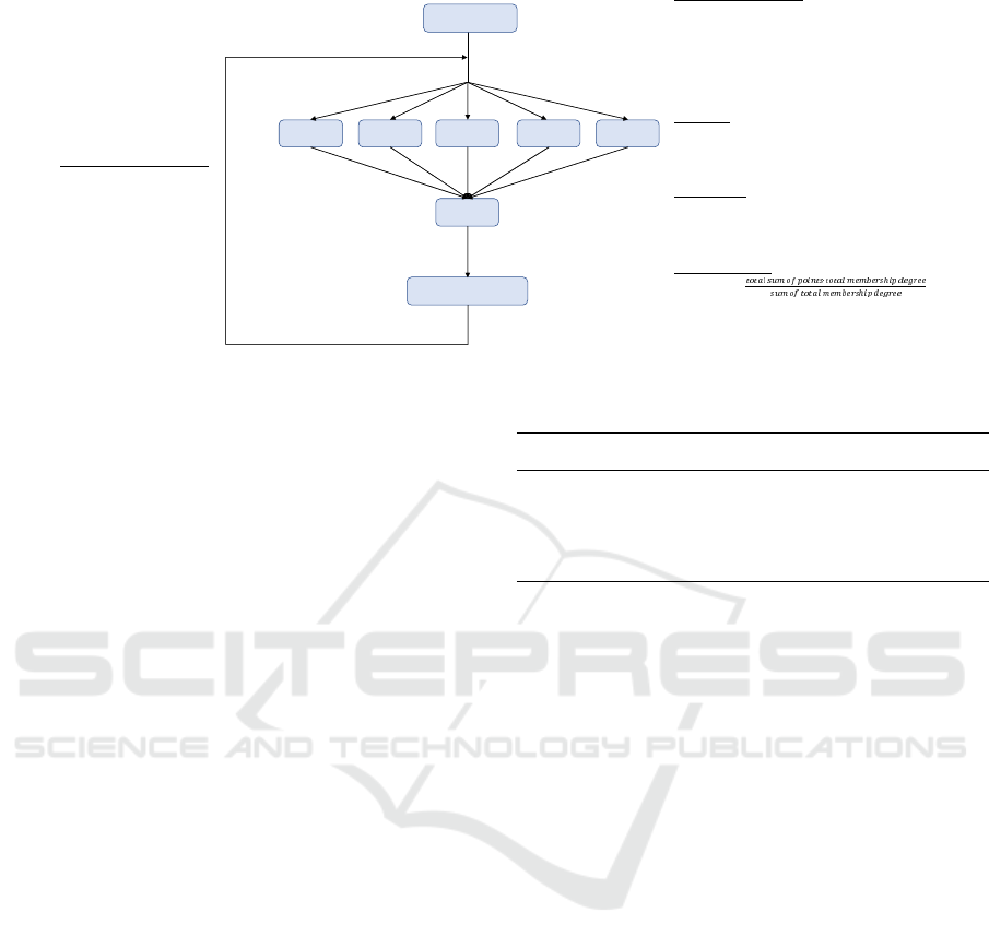
The clustering stage is composed of the following
steps, executed repeatedly until convergence is found,
as shown in Figure 1:
1. Initialization of the Centroids: The first process
that takes place is the establishment of the initial
centroids. In this process, the following are cho-
sen from a random selection of the data, in ad-
dition we should take special care not to choose
elements that contain values lost.
2. Map Phase: The next process that takes place is
the mapping phase, where the mapPartition func-
tion is used to split the data in different partitions.
In each partition and for each data of the same
one, we calculate the nearest centroid and then we
carry out two operations. On the one hand we in-
crease in one the counter that indicates the number
of elements that belong to a centroid. On the other
hand we add that data to the cumulative sum of the
cluster data represented by the centroid. For each
partition, we will obtain an array of Kx2(K rep-
resents the number of centroids) and where each
represents a cluster with the number of elements
that belong to that cluster and the sum of the vec-
tors of all those elements.
3. Reduce Phase: In the next stage of reduction we
group the results of each one of the partitions, in
such a way that when nalizar the stage reduces we
have the sums of the different counters and the
sum of vectors but for the entire dataset.
A First Approach on Big Data Missing Values Imputation
317

Map Map Map MapMap
Reduce
Centroid update
Inicialization
Centroid
inicialization
Random selection of
centroids from examples in
the dataset
Map step
Data partition
Computation per cet roid : [no. of
points, sum of points]
Reduce step
Grouping of [total no. of points,
total sum of points]
Centroid Update
New centroid =
!"! #$% &'(%")%*"+,!&
!"! #$ %," .")%*"+ ,!&
Repeat until
convergence
Repeat until there is little or no
change to centroids
Figure 1: Big Data K-means Imputation outline.
4. Centroid Update: Once obtained the information
on the centroids, we proceed to update it. For it
we will use the two data on the centroids obtained
in the previous phases. To obtain the new centroid
we divide the vector resulting from the sum of the
data that belong to the cluster by the number of
elements of the same, in this way the centroid will
be readjusted and placed at the midpoint accord-
ing to the elements that belong to the cluster it
represents.
Steps 2 to 4 are repeated until the centroids con-
verge. The convergence is evaluated by comparing
the “movement” differences of the centroids between
iterations with a given threshold.
Once the centroids have been obtained, we pro-
ceed with the imputation stage of the data that have
lost values. We go through all the examples, detecting
those with MVs, determining which cluster it belongs
to, and therefore the centroid that represents it.
Once the centroid that represents the example with
lost values is obtained, we replace those missing val-
ues with the corresponding attributes belonging to the
centroid.
3.2 Big Data Fuzzy K-means
Imputation
Big Data Fuzzy K-means Imputation (BD-FKMI) is
based on the fuzzy version of K-means, which im-
plies that the examples will belong to all centroids but
with a given membership degree. If we consider the
differences among KMI and FKMI, we must point out
two of them before describing our proposal:
• Updating the centroids must consider all exam-
ples, not only those that are the closest to it. As a
result, from each point we get, instead of the near-
est centroid index, a vector of degrees of belong-
ing, where each element of the vector corresponds
to the membership degree that has that point with
each centroid.
• The data structure we have to calculate for each
centroid is no longer [no of points, cumulative
sum of points], but, following the formula of
the diffuse grouping algorithm, we calculate for
each centroid [sum of degrees, cumulative sum of
points × corresponding degree to the centroid].
The algorithm follows the same structure and the
same series of processes than BD-KMI, but we need
to take into account the aforementioned differences
into the Map step. We describe the main algorith-
mic steps next, by following the schemata presented
in Figure 2. The membership calculation is the same
as the carried out in (Li et al., 2004) and for the sake
of brevity we will not reproduce entirely here.
1. Initialization of the Centroids: Just like KMI,
the initial centroids are randomly selected.
2. Map Phase: For each example in each partition
we compute a vector that represents the member-
ship degree to each of the centroids. In this case
the result of the execution of each partition will
result in a K × 2 matrix where the information of
each centroid is, (i) the sum of all membership de-
grees for each example and; (ii) the sum of each of
these data multiplied by its corresponding mem-
bership degree.
3. Reduce Phase: We group the results of each of
the partitions to obtain information on the total of
the data.
4. Centroid Update: We divide the sum of the data
by the sum of the degrees respect to each centroid.
IoTBDS 2019 - 4th International Conference on Internet of Things, Big Data and Security
318
DĂƉ DĂƉ DĂƉ DĂƉDĂƉ
ZĞĚƵĐĞ
ĞŶƚƌŽŝĚ ƵƉĚĂƚĞ
/ŶŝĐŝĂůŝnjĂƚŝŽŶ
ĞŶƚƌŽŝĚ ŝŶŝĐŝĂůŝnjĂƚŝŽŶ
ZĂŶĚŽŵ ƐĞůĞĐƚŝŽŶ ŽĨ ĐĞŶƚƌŽŝĚƐ
ĨƌŽŵ ĞdžĂŵƉůĞƐ ŝŶ ƚŚĞ ĚĂƚĂƐĞƚ
DĂƉ ƐƚĞƉ
ĂƚĂ ƉĂƌƚŝƚŝŽŶ
ŽŵƉƵƚĂƚŝŽŶ ƉĞƌ ĐĞƚƌŽŝĚ͗ ƐƵŵ ŽĨ
ŵĞŵďĞƌƐŚŝƉ ĚĞŐƌĞĞƐ͕ ƐƵŵ ŽĨ
ƉŽŝŶƚƐΎŵĞŵďĞƌƐŝƉ ĚĞŐƌĞĞ
ZĞĚƵĐĞ ƐƚĞƉ
'ƌŽƵƉŝŶŐ ŽĨ ƐƵŵ ŽĨ ƚŽƚĂů
ŵĞŵďĞƌƐŚŝƉ ĚĞŐƌĞĞ͕ ƚŽƚĂů ƐƵŵ ŽĨ
ƉŽŝŶƚƐΎƚŽƚĂů ŵĞŵďĞƌƐŚŝƉ ĚĞŐƌĞĞ
ĞŶƚƌŽŝĚ hƉĚĂƚĞ
EĞǁ ĐĞŶƚƌŽŝĚ с
ZĞƉĞĂƚ ƵŶƚŝů ĐŽŶǀĞƌŐĞŶĐĞ
ZĞƉĞĂƚ ƵŶƚŝů ƚŚĞƌĞ ŝƐ ůŝƚƚůĞ Žƌ ŶŽ
ĐŚĂŶŐĞ ƚŽĐĞŶƚƌŽŝĚƐ
Figure 2: Big Data Fuzzy K-means Impute outline
Steps 2 to 4 are repeated until the convergence of
the centroids is attained, in a similar fashion to BD-
KMI.
4 EXPERIMENTAL ANALYSIS
In this section we experimentally validate the pro-
posed algorithms with some well-known Big Data
benchmark datasets. Section 4.1 describes the exper-
imental framework used in our experiments. Section
4.2 is devoted to the analysis of the experiments’ re-
sults. Finally, Section 4.3 will present the computa-
tion times for the compared approaches.
4.1 Experimental Framework
In order to compare the different techniques, we have
considered three well-known Big Datasets, which fol-
lows:
• Susy: It has about 4 million instances with 19
attributes. The data have been obtained through
Monte Carlo simulations. The first 8 attributes are
kinematic properties measured by the particle de-
tectors on the accelerator while the last ten char-
acters are functions of the first 8 attributes.
• Higgs10: It has approximately 880 thousand in-
stances of 29 attributes each. As the previous
dataset was obtained through the Monte Carlo
method in the experimentation on subatomic par-
ticles.
• ECBDL14: The latest dataset is the largest one.
In the beginning it was devised for the prediction
of protein structure, and it was originally gener-
ated to train a predictor related to contact map pre-
diction in the CASP9 competition for ECBDL’14
Table 1: Parameters for the classifiers.
Classifier Parameters
DT depth: 20, maxBins: 20
RF numTrees: 20, depth: 20, maxBins: 20
ANN epochs: 50, layers: 2
neuronsLayer1: 18, neuronsLayer2: 2
conference. It has 2 million instances and 631 at-
tributes.
Since the aforementioned datasets do not contain
MVs, we will artificially induce missing data in them
following a MCAR schema. The only restriction ap-
plied is to induce only one MV per example, which
would be more representative of MCAR (since hav-
ing more MVs in some instances would be related to
a MAR schema). The amount of MVs induce will
be 5, 10 and 30%, ranging from a low to highly MV
scenario.
As we have previously mentioned, there is no
other non-na
¨
ıve imputation technique in Big Data.
Thus, we are limited to compare our two proposed
techniques either with:
• Deleting or ignoring the examples with MVs,
named as IC.
• Imputation by the mean value of each input at-
tribute, named as MC.
These two techniques are easily implemented in
Spark by using filter to detect the missing values and
the native functions to compute the cumulative sum-
mation of values in order to compute the mean value.
We want to evaluate how the imputation of the
compared techniques affects the performance of the
classifiers that would be used afterwards. To properly
evaluate such impact, we have selected some repre-
sentative classifiers from MLib, which follows: de-
A First Approach on Big Data Missing Values Imputation
319

Table 2: Accuracy results for Susy dataset.
5% of missing values 10% of missing values 30% of missing values
DT(Acc) RF(Acc) ANN(Acc) DT(Acc) RF(Acc) ANN(Acc) DT(Acc) RF(Acc) ANN(Acc)
BD-KMI(k=5) 0.782447 0.799291 0.783058 0.784201 0.799192 0.782340 0.787823 0.798408 0.780787
BD-KMI(k=15) 0.782540 0.799369 0.781930 0.784022 0.799221 0.781861 0.787458 0.798824 0.781265
BD-KMI(k=30) 0.781936 0.799334 0.781498 0.783486 0.799293 0.782304 0.786973 0.798929 0.781072
BD-FKMI(k=5) 0.781641 0.799301 0.782231 0.782242 0.799202 0.780907 0.782855 0.798951 0.782452
BD-FKMI(k=15) 0.781594 0.799348 0.781792 0.781486 0.799240 0.780951 0.782891 0.799054 0.782373
BD-FKMI(k=30) 0.781641 0.799245 0.781943 0.782154 0.799250 0.780796 0.783080 0.798977 0.782401
MC 0.781722 0.799384 0.782297 0.782090 0.799349 0.781459 0.782357 0.799070 0.782087
IC 0.780501 0.798985 0.781928 0.780040 0.799344 0.782029 0.777843 0.799021 0.782057
Table 3: Accuracy results for Higgs dataset.
5% of missing values 10% of missing values 30% of missing values
DT(Acc) RF(Acc) ANN(Acc) DT(Acc) RF(Acc) ANN(Acc) DT(Acc) RF(Acc) ANN(Acc)
BD-KMI(k=5) 0.683908 0.738168 0.628632 0.683232 0.737928 0.628159 0.682132 0.736913 0.628458
BD-KMI(k=15) 0.684011 0.738520 0.628272 0.683273 0.738078 0.627418 0.682167 0.736360 0.628511
BD-KMI(k=30) 0.684859 0.738268 0.627457 0.683835 0.737781 0.628733 0.682639 0.735936 0.628422
BD-FKMI(k=5) 0.684150 0.738195 0.627073 0.684333 0.737652 0.628078 0.682935 0.736784 0.628576
BD-FKMI(k=15) 0.684551 0.737827 0.627108 0.684171 0.737634 0.628078 0.683145 0.737112 0.628576
BD-FKMI(k=30) 0.683248 0.738243 0.627617 0.683639 0.738264 0.628078 0.683178 0.736725 0.628575
MC 0.684455 0.738275 0.627280 0.683708 0.737812 0.627210 0.681988 0.736915 0.628594
IC 0.682120 0.737390 0.627537 0.682118 0.736260 0.628446 0.675251 0.732435 0.628260
cision tree (DT), Random Forest (RF), and an artifi-
cial neural network (ANN). The parameters used for
these classifiers have been experimentally adjusted
for the original datasets to obtain a good performance
by means of grid search, and then later applied to the
imputed version of the same datasets. The obtained
parameters can be found in Table 1. Both BD-KMI
and BD-FKMI only require to specify the number of
centroids k. For both imputation techniques we will
consider k = 5, 15, 30% We have used a 5-fcv valida-
tion to validate our proposals.
For all experiments we have used a cluster com-
posed of 20 computing nodes and one master node.
The computing nodes hold the following character-
istics: 2 processors x Intel Xeon(R) CPU E5-2620,
6 cores per processor, 2.00 GHz, 2 TB HDD, 64
GB RAM. Regarding software, we have used the fol-
lowing configuration: Hadoop 2.6.0-cdh5.4.3 from
Cloudera’s open source Apache Hadoop distribu-
tion, Apache Spark and MLlib 1.6.0, 460 cores (23
cores/node), 960 RAM GB (48 GB/node).
4.2 Accuracy Analysis with the
Imputation Methods
In this section we will analyze the results obtained by
the classification methods once the imputation meth-
ods have been applied for each dataset individually.
Table 2 presents the results for the Susy dataset.
From the results presented, the best imputation tech-
nique is BD-KMI, where in most cases it performs
best with few clusters. On the other hand, we must
stress that mean imputation (MC) is the best tech-
nique for RF. Due to the fact that MC maintains the
variance of the attribute, which RF can exploit better
thanks to its sampling. Thus, a multi-classifier with
the capability of generating diverse base classifiers
could be more robust to na
¨
ıve methos as MC. Nev-
ertheless, BD-KMI is the second best to RF, being the
most balanced option for Susy.
In Table 3 we show the results for Higgs dataset.
In this case, there is a clear domain of imputation
based in clustering. In general, the FKMI imputter
offers better results for datasets with high percentages
of missing values. However, for lower percentages of
missing values, BD-KMI obtains the best precision
scores. For this dataset, MC does not achieve the high
performance that was observed for RF in Susy.
Finally, Table 4 depicts the accuracy results in the
case of ECDBL’14 dataset. Observing the results,
BD-FKMI offers better results. As for the number of
centroids, it appears that BD-KMI gives better perfor-
mance with higher k, while in the case of BD-FKMI
this value varies to a greater extent. Comparing our
proposal with MC, the latter only out-stands (with a
narrow margin) when the number of MVs is medium
to high and only for DT. Thus, the option of using
imputation-based techniques is the safest option for
ECDBL’14 dataset.
As a general analysis, we can consider that the
proposed imputation methods outperform both MC
and IC. We must stress that deleting examples with
IoTBDS 2019 - 4th International Conference on Internet of Things, Big Data and Security
320

Table 4: Accuracy results for ECDBL’14 dataset.
5% of missing values 10% of missing values 30% of missing values
DT(Acc) RF(Acc) ANN(Acc) DT(Acc) RF(Acc) ANN(Acc) DT(Acc) RF(Acc) ANN(Acc)
BD-KMI(k=5) 0.980086 0.980233 0.980234 0.980083 0.980230 0.980233 0.980105 0.980234 0.980234
BD-KMI(k=15) 0.980067 0.980231 0.980232 0.980090 0.980235 0.980234 0.980100 0.980234 0.980234
BD-KMI(k=30) 0.980079 0.980234 0.980234 0.980078 0.980236 0.980235 0.980101 0.980233 0.980234
BD-FKMI(k=5) 0.980105 0.980233 0.980234 0.980101 0.980233 0.980235 0.980106 0.980236 0.980232
BD-FKMI(k=15) 0.980095 0.980232 0.980236 0.980090 0.980235 0.980235 0.980099 0.980227 0.980234
BD-FKMI(k=30) 0.980096 0.980231 0.980232 0.980109 0.980231 0.980233 0.980103 0.980237 0.980237
MC 0.980104 0.980233 0.980235 0.980126 0.980226 0.980235 0.980153 0.980229 0.980233
IC 0.980079 0.980231 0.980234 0.980037 0.980232 0.980234 0.980065 0.980234 0.980234
MVs (IC) is never the best option, and thus we are
being able to recover part of the information lost in
all scenarios, from low to high amount of MVs.
As for which version of the clustering based im-
putation we should choose, the choice depends on the
dataset. For instance, Susy dataset favors BD-KMI,
while for the two other datasets, we get better results
when using BD-FKMI. The number of centroids cho-
sen depends on the dataset as well. However, this is
a known feature of the original K-means clustering
technique and therefore, such behavior is inherited by
the imputation methods.
4.3 Running Times Analysis
In this section we present the running times for the
imputation methods and the impact that the number of
chosen centroids have in the performance. Figures 3a
to 3c depict the running times in minutes for each ap-
proach compared in the three benchmark datasets. As
we may appreciate, the fuzzy version BD-FKMI is
slower than its crisp version BD-KMI for the same
value of k. This overhead is a logical consequence of
the membership calculation for all the centroids that
BD-FMKI carries out and was also present in the non
Big Data version of both imputation methods.
We may also appreciate that IC has a running time
of almost zero in all cases. Since IC was implemented
with a native filter of Spark, its efficiency is very high.
However, we have shown in the previous section that
IC is never the best option to deal with MVs.
MC is also very efficient and not depends on the
amount of MVs. Since the implementation of MC
implies the cumulative sum of all observed values in
the Map phase and the later division in the Reduce
step, the number of MVs will affect little to the sum
carried out. Again, MC is a very simple method that
will run fast, but we have also shown that it is rarely
the best option.
Both BD-KMI and BD-FKMI increase their run-
ning times as the number of MVs increase as the num-
ber of imputations carried out will increase with the
number of MVs. Increasing the number of centroids
k has a negative impact in the performance. However,
as occurs for Higgs dataset, the number of k can be too
high, causing a premature stagnation in the clustering
process and thus ending the process before reaching
the max number of iterations.
5 CONCLUSIONS
Two imputation techniques for MVs have been im-
plemented in Big Data that, although simple, consti-
tute a good starting point for futures developments of
the same type. Although Spark offers the machine
learning library (MLlib), it is in continuous growth
and lacks many algorithms important for the treat-
ment of MVs. The two implemented techniques of-
fer robust and efficient results for Big Data datasets,
offering reasonable execution times. Both imputation
methods surpass in most cases other two classic tech-
niques of treatment of MVs, such as mean imputation
and elimination of the instances with lost values. It is
it is important to highlight the fact that both BD-KMI
and BD-FKMI outperform the method of eliminating
instances with MVs, since this will prevent a possible
loss of valuable information.
Regarding to the performance difference between
the two proposed imputation methods, experiments
show that BD-FKMI provides better results for high
percentages of MVs in the dataset, while the BD-
KMI performs better for dataset with lower amounts
of MVs. One of the aspects that we wanted to deeper
analyze is the influence of the number of centroids.
The results show that the influence of this parame-
ter is very dependent of the dataset. The increase in
the number of centroids in our experiments will not
always improve accuracy results. On the other hand,
this increase has impact on computational time, which
is why we have not reached higher k values in our ex-
periments.
As a future work, we intend to implement a
smarter way to select the initial centroids, which has
a great impact in the solution found by any K-means
variant. An additional improvement that we will con-
A First Approach on Big Data Missing Values Imputation
321
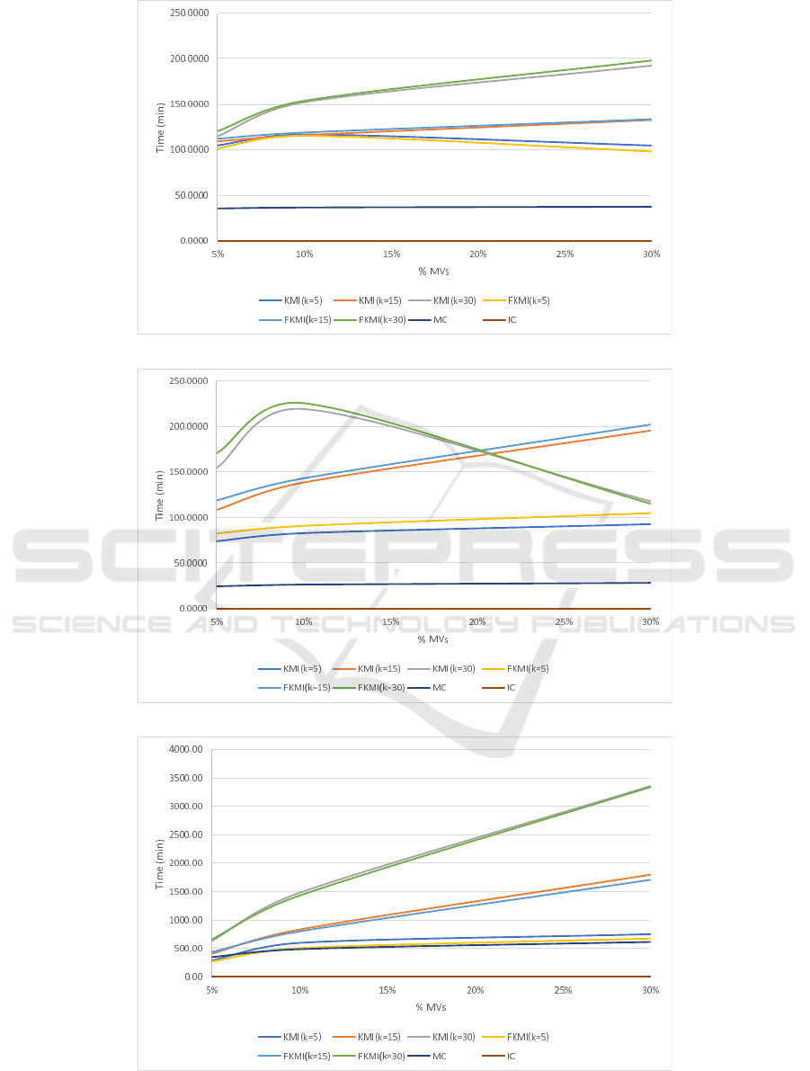
(a) Running times in minutes for Susy dataset
(b) Running times in minutes for Higgs dataset
(c) Running times in minutes for ECDBL’14 dataset.
Figure 3.
IoTBDS 2019 - 4th International Conference on Internet of Things, Big Data and Security
322

sider will be changing how the MVs are imputed. In-
stead of taking the reference attribute’s value from
the centroid, we will consider the use of a k-nearest
neighbor imputation among the closest examples in
the cluster, which may yield a closer imputed value
instead of always taking centroid’s attribute value.
ACKNOWLEDGEMENTS
This work has been supported by the project
TIN2017-89517-P granted by Ministerio de Ciencia,
Innovaci
´
on y Univesidades.
REFERENCES
Fr
´
enay, B. and Verleysen, M. (2014). Classification in the
presence of label noise: A survey. IEEE Trans. Neural
Netw. Learning Syst., 25(5):845–869.
Garc
´
ıa, S., Luengo, J., and Herrera, F. (2015). Data prepro-
cessing in data mining. Springer.
Garc
´
ıa-Laencina, P. J., Sancho-G
´
omez, J.-L., and Figueiras-
Vidal, A. R. (2010). Pattern classification with miss-
ing data: A review. Neural Computing and Applica-
tions, 19(2):263–282.
Gupta, P., Sharma, A., and Jindal, R. (2016). Scal-
able machine learning algorithms for big data analyt-
ics: a comprehensive review. Wiley Interdisciplinary
Reviews: Data Mining and Knowledge Discovery,
6(6):194–214.
Iafrate, F. (2014). A Journey from Big Data to Smart Data,
pages 25–33. Springer International Publishing.
John Walker, S. (2014). Big data: A revolution that will
transform how we live, work, and think.
Kaliamoorthy, S. and Bhanu, S. M. S. (2018). Multiple
imputation inference for missing values in distributed
datasets using apache spark. In International Confer-
ence on Advances in Computing and Data Sciences,
pages 24–33. Springer.
Kim, H., Golub, G. H., and Park, H. (2004). Missing
value estimation for DNA microarray gene expression
data: local least squares imputation. Bioinformatics,
21(2):187–198.
Laney, D. (2001). 3d data management: Controlling data
volume, velocity and variety. META group research
note, 6(70):1.
Li, D., Deogun, J., Spaulding, W., and Shuart, B. (2004).
Towards missing data imputation: a study of fuzzy k-
means clustering method. In International conference
on rough sets and current trends in computing, pages
573–579. Springer.
Little, R. J. A. (1988). A test of missing completely
at random for multivariate data with missing val-
ues. Journal of the American Statistical Association,
83(404):1198–1202.
Little, R. J. A. and Rubin, D. B. (2014). Statistical analysis
with missing data, volume 333. John Wiley & Sons.
Luengo, J., Garc
´
ıa, S., and Herrera, F. (2012). On the
choice of the best imputation methods for missing val-
ues considering three groups of classification meth-
ods. Knowledge and Information Systems, 32(1):77–
108.
Petrozziello, A., Jordanov, I., and Sommeregger, C. (2018).
Distributed neural networks for missing big data im-
putation. In 2018 International Joint Conference on
Neural Networks (IJCNN), pages 1–8. IEEE.
Qu, Z., Yan, J., and Yin, S. (2016). Association-rules-based
data imputation with spark. In 2016 4th International
Conference on Cloud Computing and Intelligence Sys-
tems (CCIS), pages 145–149. IEEE.
Ram
´
ırez-Gallego, S., Fern
´
andez, A., Garc
´
ıa, S., Chen, M.,
and Herrera, F. (2018). Big data: Tutorial and guide-
lines on information and process fusion for analyt-
ics algorithms with mapreduce. Information Fusion,
42:51–61.
Royston, P. et al. (2004). Multiple imputation of missing
values. Stata journal, 4(3):227–41.
Schneider, T. (2001). Analysis of incomplete climate data:
Estimation of mean values and covariance matrices
and imputation of missing values. Journal of climate,
14(5):853–871.
Triguero, I., Garc
´
ıa-Gil, D., Maillo, J., Luengo, J., Garc
´
ıa,
S., and Herrera, F. (2018). Transforming big data into
smart data: An insight on the use of the k-nearest
neighbors algorithm to obtain quality data. Wiley In-
terdisciplinary Reviews: Data Mining and Knowledge
Discovery, page e1289.
Zaharia, M., Xin, R. S., Wendell, P., Das, T., Armbrust,
M., Dave, A., Meng, X., Rosen, J., Venkataraman, S.,
Franklin, M. J., et al. (2016). Apache spark: a unified
engine for big data processing. Communications of
the ACM, 59(11):56–65.
A First Approach on Big Data Missing Values Imputation
323
