Monitoring Local Shoreline Changes by Integrating UASs, Airborne

LiDAR, Historical Images and Orthophotos

Gil Gonçalves

1,2

, Sara Santos

, Diogo Duarte

and José Gomes

1,4

University of Coimbra, Portugal

Institute for Systems Engineering and Computers at Coimbra, Portugal

Faculty of Geo-Information Science and Earth Observation (ITC), The Netherlands

Centre of Studies on Geography and Spatial Planning, Portugal

Keywords: Coastline Erosion, Local Change Rate, Drones, DSM, DSAS, GIS.

Abstract: Shorelines are continuously changing in shape and position due to both natural and anthropogenic causes.

The present paper is a two-fold goal: 1) analyse the relevance of low-cost UAS (Unmanned Aerial Systems)

imagery for local shoreline monitoring and control of topo-morphological changes by using the derived

Digital Surface Models (DSM) and orthophotos; 2) integrating this 2.5D and 2D geospatial data with airborne

LiDAR, historical images and national orthophotos series to assess the Furadouro’s beach erosion and

shoreline change between 1958 to 2015. Digital Surface Models (DSM) derived from airborne LiDAR and

low cost UAS are used to delineate the shoreline position for the years 2011 and 2015. A time series of

shoreline positions is then obtained by combining the shoreline obtained from the DSM and LiDAR data with

historical shoreline positions recovered from aerial images and orthophotos for the years 1958, 1998 and

2010. The accretion and erosion rates, generated by using the Digital Shoreline Analysis System (DSAS),

shows that the integration of the several Geospatial technologies was very effective for monitoring the

shoreline changes occurred in this 57-year interval, reveling an average shoreline retreat of -2.7 m/year. In

addition, the DSMs derived from UAS technology can also be effectively used in the topographic monitoring

of the primary dunes or in other processes associated with the coastline erosion phenomena.

1 INTRODUCTION

Over the years, population growth in coastal areas has

been increasing, concentrating in such locations

economic, political and social centres. This growth

was very swift and poorly planned, creating urban and

industrial pressures. Consequently, we’ve had several

coastal environments destroyed, which have caused

the increase in territorial vulnerability to coastal

erosion processes.

In this extremely dynamic context, the shoreline

continuously changes its position and shape through

time. To map the temporal evolution of the shoreline

it is necessary to consider a spatial feature (or a

shoreline proxy) that is coherent in space and time in

order to reduce the positional uncertainty (Cenci et

al., 2017). The literature concerning this issues

reveals the existence of several shoreline proxies

(e.g. mean low of water line, base/top of bluff/cliff,

vegetation line, etc.) and mapped using multi-

temporal geospatial data sources, such as satellite

imagery, historical air photos, orthophotos series,

LiDAR data, GPS profiles, etc. (Albuquerque et al.,

2013; Cenci et al., 2017; Moore, 2000; Sousa et al.,

2018).

Different geospatial technologies have also been

used to monitor foredunes and shoreline changes at a

local scale. Among these technologies we can refer:

i) the use of Airborne LiDAR combined with aerial

imagery and Global Navigation Satellite Systems

(GNSS) data for the quantification of the deflation

and horizontal migration of a group of active dunes in

the United States (Hardin et al., 2014); ii) the use of

Network Real Time Kinematics (NRTK) positioning

technologies, supported by active regional GNSS

networks to monitor at a local scale the morphology

changes of a group of dunes due to erosion and

accretion (Garrido et al., 2013); iii) the comparison

of UAS aerial imagery and its derived 3D models

through dense image matching with terrestrial laser

scanner (Gonçalves et al., 2018; Mancini et al., 2013).

In both cases, 3D data used in this approach has a

126

Gonçalves, G., Santos, S., Duarte, D. and Gomes, J.

Monitoring Local Shoreline Changes by Integrating UASs, Airborne LiDAR, Historical Images and Orthophotos.

DOI: 10.5220/0007744101260134

In Proceedings of the 5th International Conference on Geographical Information Systems Theory, Applications and Management (GISTAM 2019), pages 126-134

ISBN: 978-989-758-371-1

vertical accuracy of 0.19 m for the Root Mean Square

Error (RMSE); iv) the use of UAV images to generate

a 3D model and determine the morphological changes

with a resolution of 10cm and vertical RMSE of 5 cm

(Gonçalves and Henriques, 2015).

As above mentioned, one of the main proposes of

the present paper is to integrate DSM data and

orthophotos, both derived from UAS

Photogrammetry, with existing geospatial data (2D

and 2.5D) for monitoring local shoreline changes.

The next section presents some of the main features

concerning the study area. This is followed by the

description of the various types of Geospatial

technologies used in this work. Details of the

accuracy of the UAS images, shoreline change

methods, the results obtained and its discussion are

thus presented in a subsequent section. Finally, a brief

synopsis and final conclusions of the paper are

presented.

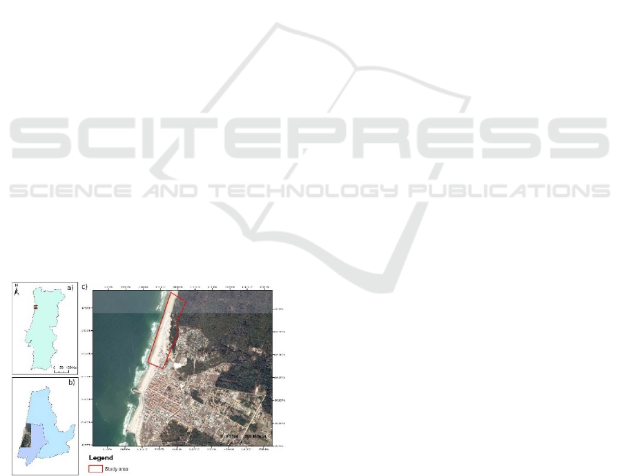
2 STUDY AREA

Furadouro’s beach is located in the northern part of

Portugal (Figure 1-a) and belongs to the county of

Ovar, an administrative region of Aveiro Portugal

(Figure 1-b). Its coastal area and morphogenic

dynamics is affected by maritime, wind and anthropic

processes. The coastal area is defined by a very

attractive and extensive sand beach suitable for

touristic activities which in turn is increasing

territorial vulnerabilities to the natural coastal

dynamics. As a consequence, a fast urbanization took

place which often covers primary dunes and directly

affects the coastal processes.

Figure 1: The study area: Furadouro’s beach.

The (geo)morphology has been showing signs of

several shoreline erosion processes, namely, those

with oceanic and windy origins. These processes have

been reducing the sandy area of the beach while the

ocean is advanced and gaining ground to the beach.

Furthermore, with the occurrence of meteorological

events, the action of such processes is accentuated.

The urbanized areas of Furadouro already present

several walled slopes on its south side, where

residents aim at temporarily protect their properties.

The recent construction of artificial bays at the north

side of the beach will also increase the severity of

these coastal processes generating more hazards and

risks in this territory.

3 GEOSPATIAL DATA AND

TECHNOLOGIES

3.1 Municipal Geospatial Data Archive

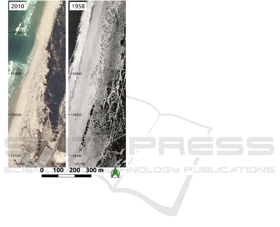
Two images of the historical United States Air Force

(USAF) 1958 flight and 3 orthophotos series were

used. These were obtained from the geospatial data

archive of the municipality of Ovar The radiometric

quality (8 bits) of these digitalized UASF images are

very poor and the camera calibration parameters are

unknown. Therefore, it was impossible to use them in

order to generate the DSM using a Structure from

Motion and Multi-View Stereo (SfM-MV)

approaches. Concerning the orthophotos they belong

to the national coverage series published by the

Portuguese Mapping Agency (Figure 2).

3.2 GNSS NRTK

The positioning survey method used for this study is

based on NRTK approach. It uses the observations of

GNSS acquired from the several Continuously

Operating Reference Stations (CORS) network

stations to model the error, at the rover, of the

spatially correlated differences (the orbital errors and

the ionospheric and tropospheric delays of the GNSS

signal). The error is modelled assuming that these are

constant for a given region. Merging the data coming

from the multi-frequency GNSS receivers with the

NRTK corrections available (national) both precision

and accuracy are superiors to the conventional RTK

(using a single network station). Furthermore the

NRTK solution offers a better coverage and

reliability, more homogeneous accuracy and is faster

when solving the ambiguities (Garrido et al., 2012).

In this work the RENEP network with the geodetic

system ETRS89, ETRF97 with year of reference

1995.4, was used. It broadcasts the differential

corrections in real time in the format RTCM 3.1.,

Monitoring Local Shoreline Changes by Integrating UASs, Airborne LiDAR, Historical Images and Orthophotos

127

which can be obtained via Internet with NTRIP

(networked transport of RTCM via internet protocol).

Network corrections using this approach allows the

generation of positional accuracy and precision at a

centimetre level (Aponte et al., 2009; Garrido et al.,

2012; Pepe, 2018).

Figure 2: Two examples of geospatial data used in this

study: the 2010 orthophoto and the 1958 image mosaic.

Ground Control Points (GCP) and cross profile

survey tasks were performed with: i) two GNNS

Geomax Zenith 10, equipped with triple frequency

antennas (GPS, GLONASS, Galileo); ii) two wireless

controlers GEOMAX PS339; iii) additional

accessories such as tripods and targets. The

planimetric coordinates (xy) of the geospatial data

were referenced to the system ETRS89 PT/TM-06

(EPSG:3763) and the z coordinate to the geoid

(orthometric altitude) using the numerical local geoid

model GEODPT08.

3.3 Airborne LiDAR

LiDAR is commonly used in large scale shoreline

mapping and change detection, due to its high

geometrical accuracy, affordable costs and

acquisition speed (Brock and Purkis, 2009). An

airborne LiDAR system is basically composed of a

laser scanner, GNSS in differential mode and Inertial

Measurement Unit (IMU). The typical data of a

LiDAR survey is an irregular point cloud with three-

dimensional coordinates where each point contains an

ID (Petrie, 2011). This ID contains a given temporal

mark and also the intensity of the received signal, the

number of the return and quantity. The intensity of the

reflected light is dependent on the surface

characteristics, wave length of the laser and the

incidence angle.

The LiDAR data used in this work is in a grid

format and with spatial resolution of 1m. It was

acquired with a LiDAR topographic LEICA ALS60

flying at a medium 1800m flight height between

November, 17

and December, 7

, 2011.

3.4 UAS Photogrammetry

The low cost profile and versatility of UAV

equipment combined with the advancements both in

computer and photogrammetry were identified in

literature (expand). The drone system is described in

Table 1.

4 METHODOLOGY

The 2.5D digital representation of the coastline using

high-resolution digital surface models, has been

intensively employed in the topographical monitoring

of coastal erosion (Mitasova et al., 2005). Such data

can be further used in the study of several shoreline

phenomena; for example, in coastal erosion

simulations, flooding and monitoring coastal

sediments (Mancini et al., 2013). The current paper,

reveals the importance of the use of digital surface

models obtained from UAV-images (dense image

matching) and aerial LiDAR data. These were used to

hand-made delineation of the coastline planimetric

position for the years 2011 and 2015. The study of

the coastal erosion has been taking advantage of high-

resolution digital surface models (2.5D). Such

information allows to perform simulations of coastal

erosion, flooding phenomena and to monitor the

balance of coastal sediments (Mancini et al., 2013).

The methodology adopted to determine shoreline

change rates involves four main steps (Figure 3): 1)

acquisition of the pertinent geospatial data for the

period under evaluation; 2) manual digitalization of

each shoreline and evaluation processes of the main

error sources that affects the shoreline measurements

in each category of geospatial data; 3) building of the

shoreline time-series geodatabase and corresponding

attribute data necessary for the GIS based DSAS

GISTAM 2019 - 5th International Conference on Geographical Information Systems Theory, Applications and Management

128

package; 4) computation of the shoreline change rates

statistics.

Table 1: UAS specifications. G.C.S and D/W are the

abbreviations for Ground Control Station and

Dimensions/Weight, respectively.

Platform

Type: Quadcopter Tarot Iron Man 650

Engine Power: 4 T-Motor Navigator MN3110 470KV

Dim./weight: 95 cm / 1.5 kg (for all equipment)

Flight mode: Manually based on wireless control

Endurance: 15 min (+ 3 min safety)

Digital camera

Support: Walkera G-2D Brusless gimbal

Camera model: GoPro Hero4 Silve

→ Sensor type CMOS - 1/2.3’’

→ Pixel pitch [m] 1.54

→ Lens Wide-angle lens

/2.8 6-element aspherical glass

→ Sensor window Narrow FOV mode (focal 34.4 mm)

D/W: 41.0x59.0x29.6 mm / 84g

Flight control system

Controller: DJI Naza V2 (GPS)

G.C.S Futaba 8J FHSS - FUTABA

2-stick, 8-channel, S-FHSS, Buil

-in

Dual Antenna Diversity

Transmitting frequency: 2.4GHz band

FPV

–

Tx/Rx: DJI Video Link 5.8Ghz 500mw

Monitor: 7” LCD

Price: Approx. 1200 € (home assembled kit)

4.1 Photogrammetric Workflow

The photogrammetric workflow used to produce the

DSM and orthophoto from the set of UAV images

was performed in 3 main steps: 1) flight planning; 2)

flight execution; 3) generation of both the DSM and

orthophoto.

Regarding the step 1) several inputs were

required. First, the ground pixel resolution (i.e.

ground sampling resolution - GSD) must be defined.

The flying height can then be determined for a given

camera. Another issue is the image overlap (frontal

80% and lateral 60%), flying speed and

corresponding shutter speed and distance between

flying lines. Finally, the GCP must be well planned to

allow a good Bundle Block Adjustment (BBA), since

the direct georeferencing using the current drone was

not possible (Rangel et al., 2018). Prior to the flying

of the drone, targets were deployed in the area and

their coordinates were acquired using a GNSS-NRTK

method. Given that the drone can only be manually

operated, a capture interval of five seconds image was

introduced in the camera settings. The flying height

was of 100m (GSD of 6 cm) and four flying lines

were defined to be flown, parallel to the coastline. To

generate the 3D model from the UAV images,

Photoscan was used. First we determined the tie

points among all the 170 images. This allowed to

calibrate the camera used in the study and to perform

the relative and absolute orientation of the image

block. This information was then used as input for the

dense image matching performed in the last step,

which gave us the final 3D point cloud. This final step

for data aquisition process enabled the computation

of the corresponding DSM and orthophoto.

4.2 Accuracy Assessment of the DSM

Derived from UAS Imagery

To assess the accuracy of the DSM derived from UAS

imagery, we plot several terrain profiles which are

perpendicular to the coast line. The DSM was then

compared with two terrain cross profiles which were

Figure 3: Workflow of the proposed methodology.

Monitoring Local Shoreline Changes by Integrating UASs, Airborne LiDAR, Historical Images and Orthophotos

129

recorded with GNSS-NRTK. For each planimetric

position of the points that define the terrain profile we

determined the height difference between the DSM

and the ones obtained with the GNSS received in

NRTK mode, henceforth referred as vertical residual.

With these differences we determined the RMSE,

mean and standard deviation.

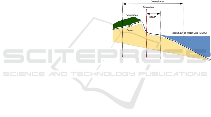
4.3 Shoreline Proxy

In the literature, coastline and shoreline concepts may

have different meanings (including in legal terms);

however, in this study, these are used interchangeably

being more conservative in spatial location than the

physical interface of land and water, the latter being

commonly used to define “shoreline”. Nevertheless,

given the extreme shoreline dynamics , its mapping is

usually based on an indicator/proxy. Considering that

our goal is to monitor low-lying sandy beaches

backed by dunes, the shoreline proxy used was the

foredune toe. This proxy is described by either a slope

break (break-line) and the seaward limit of

vegetation, which are mainly covered by scattered

vegetation (Figure 4). It is recognized as the

morphological coastal feature less affected by short-

term (tidal) and medium-term (seasonal) changes and

was also used in previous studies (Ponte Lira et al.,

2016), which mapped 92% and 95% of all the low-

lying sandy beaches of mainland Portugal for the

years 1958 and 2010, respectively.

In this work the two DSMs derived from LiDAR

and UAS, were used as a base for the manual

delineation of the planimetric position of the coastline

for the years of 2011 and 2015 respectively. With the

help of DSM hillshading techniques, it was possible

to manual delineate the breaklines, corresponding to

the position of the foredune toe.

4.4 Monitoring Shoreline Changes

Available for ArcGIS, the DSAS tool, allows the

automation of processes that are required for the

quantitative analysis of the evolution of a timeseries

of shoreline data. Using equidistant terrain profiles

delineated in GIS environment, these profiles were

intersected with intersected with the shoreline of each

epoch. These intersections were then used by several

statistical methods to determine the increase/not-

increase rates in the coastal erosion complex process.

In this work, we used the End Point Rate (EPR)

the Linear Regression Rate (LRR) and the Weighted

Linear Regression (WLR) methods. The EPR method

determines the variation of the coastline dividing the

distance of the coastal line movement by the time

going from the oldest to the most recent line (Thieler

et al., 2009). The LRR method determines the retreat

rate of the coastline using a simple linear regression,

considering the variations present along each defined

coastline. In this case, all the terrain profiles were

considered in the statistical computations. However,

these method tends to underestimate the rate of

variation when compared with other statistical

measures and its susceptible to extreme deviations

(Thieler et al., 2009). Therefore, the WLR method

tends to smooth the data by giving more emphasis or

weight to the geospatial data for which the positional

uncertainty is smaller. This weight (w) is usually

defined as a function of the variance in the uncertainty

of the measurement (e), that is: w = 1/ (ut2), where ut

is the shoreline uncertainty value.

Figure 4: Shoreline proxy.

Moreover, it is possible to obtain some

complementary measures, such as, the correlation

coefficient, confidence interval and adjustment error.

4.5 Estimation of the Positional

Uncertainty

Each geospatial mapping technology has its own

sources of uncertainty, which in turn, affect the

estimation of the shoreline change rate. These

uncertainties are usually grouped in two categories

(Fletcher et al., 2003): i) the measurement

uncertainty, which is related to the characteristics of

the data source technology and the operator-based

measurement method; ii) the modeling (geometric

representation of the shoreline) uncertainty which is

related to all factors and phenomena that affect the

spatial position of the real shoreline during a given

year (e.g., stage of the tide, recent storms, seasonal

state of the beach). In this study, the chosen shoreline

proxy was affected by the following measurement

uncertainties:

 Digitizing uncertainty (u

) – represents the uncer-

GISTAM 2019 - 5th International Conference on Geographical Information Systems Theory, Applications and Management

130

tainty produced by the operator due to some

difficulties related to the visual interpretation of

the shoreline. It was evaluated by digitizing

several times the same shoreline on the same

image,

 Resolution uncertainty (u

) – represents the

smallest feature that is theoretically possible to

identify on the geospatial product (image, ortho,

DSM),

 Planimetric uncertainty (u

) – represents the

horizontal accuracy that characterizes each

specific source of data. For image data it was

chosen the RMSE of the check points used in the

registration process. For the orthophotos it was

given by the RMSE of the aerotriangulation

process and the published accuracy figures for

each data set. For the case of surface data

(LiDAR-based DSM and UAS-based DSM) the

effect of the altimetric uncertainty (σ

) was also

taken into account on the planimetric (σ

)

uncertainty by using the mean slope (tan



) of the

surface in the vicinity of the shoreline (Kraus,

1994):









tan

⁄

(1)

Assuming that these uncertainties are random and

uncorrelated the total uncertainty quantified by

calculating the square root of the sum of the squares

of all uncertainties:



























(2)

Table 2 shows these uncertainties for each shoreline

epoch. The uncertainty related with the digitalization

of the shoreline (u

) was evaluated as the RMSE of

the digitalization process carried out by 3 different

operators.

5 RESULTS AND DISCUSSION

The proposed methodology for acquiring reliable

shoreline information was implemented using the

available UAS technology for the year 2015.

5.1 DSMs Derived from LiDAR and

UAS

Figure 5 (a and b) shows, respectively, the orthophoto

and DSM (0.10 m resolution) obtained by the UAS

technology and used in the manual delineation of the

coastline for the year 2015. Figure 5-c shows the

DSM (1m resolution) obtained with LiDAR

technology and used in the manual delineation of the

2011 coastline.

Figure 5: Ortophoto (a) and DSM (b) obtained from UAS

imagery (2015); (c) DSM obtained from LiDAR (2011).

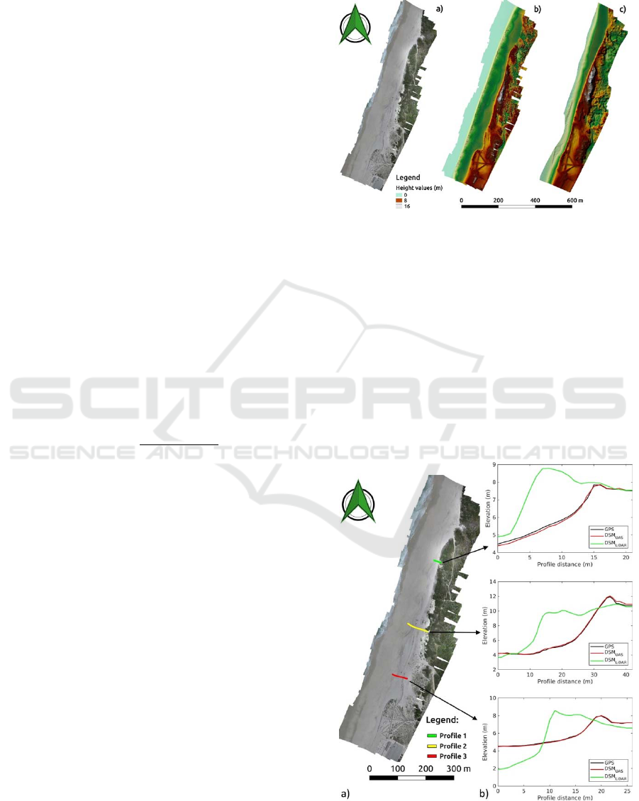
5.2 Accuracy Assessment of the DSM

Derived from UAS Imagery

In Figure 6-a it can be seen the location of the three

terrain profiles obtained by the GNSS-NRTK survey.

Although these profiles are used for assessing the

vertical accuracy of the DSM obtained by the UAS,

these terrain profiles can also be used to observe the

dynamics of Furadouro’s beach for the period 2011-

2015, when compared with the corresponding profiles

interpolated from the DSM-LiDAR (Figure 6-b).

Figure 6: Location of the transversal profiles used to assess

the vertical accuracy. b) Comparative analysis.

Monitoring Local Shoreline Changes by Integrating UASs, Airborne LiDAR, Historical Images and Orthophotos

131

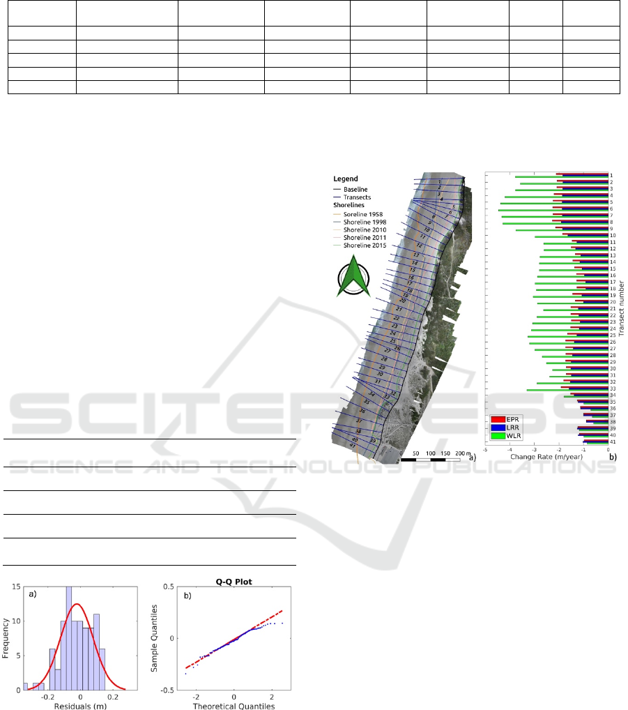
Table 2: Uncertainty (uncert,) measures.

Shoreline

epoch

Acquisition

technolog

Digitalization

mode

Spatial

resolution

Digitizing

uncert.

Resolution

uncert.

Plan.

uncert.

Total

uncert.

1958 Film camera Air photo ≈ 85 cm/pix 6 pix 2 pix 7.0 m 4.30

1998 Film camera Ortho ≈ 50 cm/pix 4 pix 2 pix 2.2 m 2.30

2010 Digital camera Ortho 50 cm/pix 2 pix 2 pix 0.7 m 0.80

2011 Airborne Lida

DSM ≈ 1 pt/m2 75 cm 1.5 pix 0.5 m 0.50

2015 UAS imagery Ortho+DSM 10 cm/pix 15 cm 1.5 pix 0.3 m 0.30

Comparing the two terrain profiles interpolated

from the DSMs obtained from the UAS techniques,

and the ones obtained directly from the GNSS-NRTK

survey, we can compute some statistical measures for

the vertical accuracy of the DSM. Table 3 illustrates

some of the statistical measures for the positional

accuracy (RMSE = 10 cm). It should be stressed that

the mean varies from positive to negative between the

profiles.

The normality of the distribution of the 92

residuals can be determined visually by two ways:

generating the histogram and superimpose it with the

normal distribution curve (Figure 7-a); or using a

quantil-quantil (Q-Q) plot (Figure 7-b). Given that the

curve of the graph Q-Q is close to the red line we can

consider that we are facing a normal distribution of

the residues, mean, RMSE and standard deviation of

10cm (1 GSD).

Table 3: Vertical accuracy indicators for UAS-DSM.

N RMSE (cm) μ (cm) σ (cm)

Profile 1 22 10 6 8

Profile 2 43 12 -9 8

Profile 3 27 5 3 5

Global 92 10 -2 10

Figure 7: Normality testing for the profile residuals; a)

Histogram with normal distribution curve; b) Q-Q plot.

5.3 Shoreline Changes

For this analysis we used the shorelines for the years

1958, 1998, 2010 and 2011, which were inserted into

a geodatabase. A baseline from the shoreline

corresponding to the year 2015 was then drawn. This

was performed by having a 15 m buffer around the

2015 shoreline.

Figure 8: Evaluating the shoreline variation rates with

DSAS: a) Location of the transects; b) Variation rates with

three metrics (EPR, LRR e WLR).

Figure 8 shows the several retreat rates (negative

values) of the shoreline for the 3 statistical measures

(LRR, EPR and WLR). From the data we can observe

that Furadouro has been through both coastal erosion

and accretion. The latter corresponds to the temporal

period 1998-2010 (profiles 15 to 37). It can also be

observed the strong retreat process of the shoreline

between 2010 and 2011, for example, profile 5 which

presents a 46 m retreat process. From profile 8, and

for the interval 1958-2015, a deeper and more evident

retreat process -128 m can be observed (which is the

maximum retreat value for the study area).

Furthermore, the LRR has lower values in all of the

profiles, exception being profiles 36 and 37. It needs

to be noted that these profiles are located in an area

already artificialized, namely with the construction of

beach accesses and other recreational facilities. The

highest mean value of the LRR corresponds to -1.9

m/year and the lowest -0.9 m/year. Concerning the

EPR, this statistical measure presents the higher rates

GISTAM 2019 - 5th International Conference on Geographical Information Systems Theory, Applications and Management

132

of erosion, where it peaks at -2.3 m/year and

minimum -0.89m/year. The mean retreat rate of the

coastline for the 57 year interval considered in this

study is of -1.5m/year. Some other figures can be

stressed, for example, -1.4m/year for the LRR, -

1.6m/year for the EPR and -2.7m/year for the WLR.

We can conclude that there was a generalized

erosional continuous and complex process in the

given time-frame. If we compare these results with

previous studies, for example (Silva, 2012) and

(Ponte Lira et al., 2016), we can conclude for the

existence of some important discrepancies. Just to

confirm this conclusion (Silva, 2012) reports the

following retreat rates: -2.7 m/year from 1958 to 2010

and -4m/year for the period 2010/2012. In spite of the

study area being larger than our study area, the time

periods and the scale of analyses are also different.

This and the reported work both present a coastal

erosion process that surpasses 1.5 m per year.

6 CONCLUSIONS

Over the last decades, the Furadouro's beach has been

suffering an increasingly severe shoreline retreat

process. The DSAS tool was very effective in

quantifying retreat rates, obtaining a mean value of -

2.7 m / year (WLR) for the study area and for the 57

year time period: 1958 to 2015. In this work the DSM

obtained by LiDAR aerial was undoubtedly an

excellent starting point for the local monitoring of

coastal erosion, since it allows for unambiguous

definition of a temporal reference concerning the

topographic position of the shoreline and the coastline

surface and migrations process. In addition, it allows

to integrate low-cost technologies (UASs) into local

monitoring shoreline procedures. By allowing the

generation of orthophotos and DSM, simultaneously,

it is an added value in studies of coastal erosion at a

local scale. Finally, it should be noted that the

integration of several geospatial technologies in the

topographic monitoring of the coastline also raises the

need to standardize the concept of the coastline

extracted from different geospatial data. As a final

comment, these conclusions allow the authors to

propose that increasing people awareness for the

importance of hazards and risks mitigation and if we

have in mind that Climate Changes are already

producing substantive land and territorial changes,

something must be done. It is our conviction that

Geospatial technologies constitute a suite of

interoperable tools that can support decision makers

in order to implement a “culture of prevention”

instead of a “culture of reaction” as it has been argued

by the UNESCO-ISDR (UNISDR, 2007).

ACKNOWLEDGEMENTS

This work was partially supported by project grant

UID/MULTI/00308/2019 and by the European

Regional Development Fund through the COMPETE

2020 Programme, FCT - Portuguese Foundation for

Science and Technology within the project

PTDC/EAM-REM/30324/2017.

REFERENCES

Albuquerque, M., Espinoza, J., Teixeira, P., de Oliveira, A.,

Corrêa, I., Calliari, L., 2013. Erosion or Coastal

Variability: An Evaluation of the DSAS and the Change

Polygon Methods for the Determination of Erosive

Processes on Sandy Beaches. J. Coast. Res. 165, 1710–

1714. https://doi.org/10.2112/SI65-289.1

Aponte, J., Xiaolin, M., Hill, C., Moore, T., Burbidge, M.,

Dodson, A., Meng, X., 2009. Quality assessment of a

network-based RTK GPS service in the UK. J. Appl.

Geod. 3, 25–34. https://doi.org/10.1515/JAG.2009.003

Brock, J.C., Purkis, S.J., 2009. The Emerging Role of Lidar

Remote Sensing in Coastal Research and Resource

Management. J. Coast. Res. 10053, 1–5.

https://doi.org/10.2112/SI53-001.1

Cenci, L., Disperati, L., Persichillo, M.G., Oliveira, E.R.,

Alves, F.L., Phillips, M., 2017. Integrating remote

sensing and GIS techniques for monitoring and

modeling shoreline evolution to support coastal risk

management. GIScience Remote Sens. 55, 1–21.

https://doi.org/10.1080/15481603.2017.1376370

Fletcher, C., Rooney, J., Barbee, M., Lim, S.C., Richmond,

B., 2003. Mapping Shoreline Change Using Digital

Orthophotogrammetry on Maui, Hawaii. J. Coast. Res.

Spec. Issue No. 38 106–124.

Garrido, M.S., Giménez, E., Armenteros, J.A., Lacy, M.C.,

Gil, A.J., 2012. Evaluation of NRTK positioning using

the RENEP and RAP networks on the Southern border

region of Portugal and Spain. Acta Geod. Geophys.

Hungarica 47, 52–65. https://doi.org/10.1556/

AGeod.47.2012.1.4

Garrido, M.S., Giménez, E., Ramos, M.I., Gil, A.J., 2013.

A high spatio-temporal methodology for monitoring

dunes morphology based on precise GPS-NRTK

profiles: Test-case of Dune of Mónsul on the south-east

Spanish coastline. Aeolian Res. 8, 75–84.

https://doi.org/10.1016/j.aeolia.2012.10.011

Gonçalves, G.R., Pérez, J.A., Duarte, J., 2018. Accuracy

and effectiveness of low cost UASs and open source

photogrammetric software for foredunes mapping. Int.

J. Remote Sens. 00, 1–19. https://doi.org/10.1080/

01431161.2018.1446568

Monitoring Local Shoreline Changes by Integrating UASs, Airborne LiDAR, Historical Images and Orthophotos

133

Gonçalves, J.A., Henriques, R., 2015. UAV

photogrammetry for topographic monitoring of coastal

areas. ISPRS J. Photogramm. Remote Sens. 104, 101–

111. https://doi.org/10.1016/j.isprsjprs.2015.02.009

Hardin, E., Mitasova, H., Tateosian, L., Overton, M., 2014.

GIS-based Analysis of Coastal Lidar Time-Series.

https://doi.org/10.1007/978-1-4939-1835-5

Kraus, K., 1994. Visualization of the quality of surfaces and

their derivatives. Photogramm. Eng. Remote Sensing

60, 457–462.

Mancini, F., Dubbini, M., Gattelli, M., Stecchi, F., Fabbri,

S., Gabbianelli, G., 2013. Using unmanned aerial

vehicles (UAV) for high-resolution reconstruction of

topography: The structure from motion approach on

coastal environments. Remote Sens. 5, 6880–6898.

https://doi.org/10.3390/rs5126880

Mitasova, H., Overton, M., Harmon, R.S., 2005. Geospatial

analysis of a coastal sand dune field evolution: Jockey’s

Ridge, North Carolina. Geomorphology 72, 204–221.

https://doi.org/10.1016/j.geomorph.2005.06.001

Moore, L.J., 2000. Shoreline mapping techniques. J. Coast.

Res. (ISSN 0749-0208) 16, 111–124.

https://doi.org/10.2112/03-0071.1

Pepe, M., 2018. CORS architecture and evaluation of

positioning by low-cost GNSS receiver. Geod. Cartogr.

44, 36–44. https://doi.org/10.3846/gac.2018.1255

Petrie, G., 2011. Airborne topographic laser scanners. GEO

Informatics 34–44.

Ponte Lira, C., Silva, A.N., Taborda, R., De Andrade, C.F.,

2016. Coastline evolution of Portuguese low-lying

sandy coast in the last 50 years: An integrated approach.

Earth Syst. Sci. Data 8, 265–278.

https://doi.org/10.5194/essd-8-265-2016

Rangel, J.M.G., Gonçalves, G.R., Pérez, J.A., 2018. The

impact of number and spatial distribution of GCPs on

the positional accuracy of geospatial products derived

from low-cost UASs. Int. J. Remote Sens. 00, 1–18.

https://doi.org/10.1080/01431161.2018.1515508

Silva, P.M.C., 2012. A tendência da linha de costa entre as

praias de Maceda e S. Jacinto. Universidade de Aveiro.

Sousa, W.R.N. de, Souto, M.V.S., Matos, S.S., Duarte,

C.R., Salgueiro, A.R.G.N.L., Neto, C.A. da S., 2018.

Creation of a coastal evolution prognostic model using

shoreline historical data and techniques of digital image

processing in a GIS environment for generating future

scenarios. Int. J. Remote Sens. 00, 1–15.

https://doi.org/10.1080/01431161.2018.1455240

Thieler, E.R., Himmelstoss, E.A., Zichichi, J.L., Ergul, A.,

2009. The Digital Shoreline Analysis System (DSAS)

Version 4.0 - An ArcGIS extension for calculating

shoreline change, Open-File Report. Reston.

UNISDR, 2007. Towards a Culture of Prevention: Disaster

Risk Reduction Begins at School [WWW Document].

URL http://www.unisdr.org/files/761_education-good-

practices.pdf (accessed 3.12.19).

GISTAM 2019 - 5th International Conference on Geographical Information Systems Theory, Applications and Management

134