Improving the Performance of Road Network Analysis:

The Morandi Bridge Case Study

Vincenzo Petito, Maurizio Leotta

and Marina Ribaudo

Dipartimento di Informatica, Bioingegneria, Robotica e Ingegneria dei Sistemi (DIBRIS), Università di Genova, Italy

Keywords:

Centrality Measures, OpenStreetMap, Multi-core Computation.

Abstract:

Road network analysis is a fundamental tool for city planners and engineers for preventing, or ﬁnding possible

solutions to, gridlock congestion and immobility. In this work, we describe the computation of some classical

centrality measures for the road network of the region Liguria, in particular focusing on the effects of the

2018 Morandi bridge collapse. Given the size of the network graph derived from the OpenStreetMap publicly-

available data, we extended the JGraphT library to support multi-core computation. In this way, it is possible

to deal with large graphs (e.g., 53743 nodes and 125250 edges for the considered case study), representing

real networks, with relevant time savings (up to -87% on the adopted conﬁguration). Results show that, on

the considered case study, even a classical measure like Betweenness centrality is able to provide interesting

insights on the road network under investigation.

1 INTRODUCTION

Urban population of the world has grown rapidly in the

last decades. According to the United Nations, in 2016

there were 7.4 billions inhabitants in the world (United-

Nations, 2016), and it is estimated that 68% of the

population will live in urban areas by 2050 (United-

Nations, 2018). Such ever-increasing urban population

requires city planners and engineers to look for ways

to analyze the road network in order to ﬁnd possi-

ble solutions to gridlock congestion and immobility.

Moreover, network planning and trafﬁc ﬂow optimiza-

tion are also particularly important to try to mitigate

air pollutant emissions, which constitute an important

environmental issue in several countries.

Urban trafﬁc analysis can be carried out by rely-

ing on different kinds of data, such as: (1) real traf-

ﬁc data, recorded using for example pneumatic road

tubes counters, piezo-electric sensors, or video vehicle

detection (Windmill, 2018), (2) population data, typ-

ically generated from survey data or thanks to tools

for mobile crowdsensing such as Waze

, (3) networks

of roads such as maps equipped with other types of

data like the number of road lanes, or the max allowed

speed of the roads, etc.

https://orcid.org/0000-0001-5267-0602

https://orcid.org/0000-0003-0697-2225

https://www.waze.com

With trafﬁc data it is possible to have a detailed

assessment of the road network status in terms of

hotspots, congestions, vehicle ﬂeet composition, and

the like, while the analysis of the network topology

allows to perform trafﬁc simulations or to answer to

questions such as “Which are the most important areas

of the road network?” or “What could happen to the

trafﬁc if the topology of the road network changes?”.

Following the second approach, e.g. analysis of

the network topology, our work started with the in-

tention of computing centrality measures of the Open-

StreetMap

(OSM) road network of the region Liguria

and the city of Genoa. For the computation we se-

lected the Java library JGraphT ﬁnding that there was

room for performance improvements, since the library

was not exploiting all possible parallelism. Moreover,

during the course of this activity, a tragic event hap-

pened in the city since on August 14th an important

bridge on the highway that passes through the city, the

Morandi bridge, collapsed (Glanz et al., 2018). Thus

we decided to investigate how this event changed the

topology and graph metrics of the underlying network.

Therefore, the contributions of this paper are the

following: (1) a description of how it is possible to

take the open data extracted from OSM and to derive

interesting information about the road topology; (2) a

reﬁnement of the JGraphT library in order to support

https://www.openstreetmap.org

Petito, V., Leotta, M. and Ribaudo, M.

Improving the Performance of Road Network Analysis: The Morandi Bridge Case Study.

DOI: 10.5220/0007745702590266

In Proceedings of the 5th International Conference on Geographical Information Systems Theory, Applications and Management (GISTAM 2019), pages 259-266

ISBN: 978-989-758-371-1

259

multi-core computation; (3) an empirical evaluation

of the beneﬁts obtained thanks to the JGraphT reﬁne-

ment; (4) a preliminary evaluation of the effects of the

Morandi bridge collapse on the characteristics of the

region Liguria road network.

The rest of the paper is organized as follows: Sec-

tion 2 describes the model of the road network that

can be obtained starting from the data available in

OSM and brieﬂy recalls some centrality metrics. In

Section 3 we present some related work and in Sec-

tion 4 we discuss the improvements applied to the

JGraphT library in order to fully exploit parallelism

and ﬁx some problems. Section 5 reports the results of

the empirical study aimed at quantifying the improve-

ments due to the JGraphT modiﬁcations, and shows

a preliminary analysis of the effects of the Morandi

bridge collapse. Finally, Section 6 concludes the work

discussing possible future directions.

2 ROAD NETWORK AND

METRICS

In order to analyse a road network we need accurate

data representing the network itself. Our choice is to

rely on OpenStreetMap since nowadays it is one of

the major sources for roads information. OSM is a

crowd-sourced project collecting extensive geographic

data such as roads, buildings, or other elements like

points of interest, shops, trafﬁc lights, etc. Indeed,

rather than the map itself, the data generated by the

project is considered its primary output: the entire

database of OSM can be freely accessed, and used

as the basis for third-parties map-based applications

or research studies that analyse roads characteristics

or use the map as a data source for trafﬁc simulation

models (Zilske et al., 2011).

2.1 OSM Graph Description

OSM data can be downloaded in different ways start-

ing from the OSM website download area

. It is pos-

sible to download the full dataset (which is huge) or

to select smaller areas. Map data are XML formatted,

stored into .osm ﬁles, and can be serialized into other

formats to be used in third-party applications.

Elements are the basic components of the OSM

conceptual data model of the physical world. They

consist of (1) nodes, deﬁning points in space, (2) ways,

deﬁning linear features (e.g., roads, rivers, etc.) and

area boundaries (e.g., buildings, forests, etc.), and

https://wiki.openstreetmap.org/wiki/Downloading_

data

(3) relations, which are used to explain how differ-

ent elements work or are connected together.

A way is a sequence of nodes and two ways inter-

sect if they share a common node. Our ﬁrst prototype

was developed by mapping intersections between ways

into graph nodes, and by connecting these nodes when

there was a way connecting them.

However, we realized that the JGraphT library sup-

ports centrality measures only for nodes and not for

edges and therefore we adopted a different graph struc-

ture, building a line graph

. Ways in OSM data be-

come nodes and there is an edge from node A to node

B if (1) the ways represented by A and B share an

intersection and (2) the orientation of the ways allows

a movement from A to B. Therefore, each node in the

graph represents a complete road or a segment, and

the resulting graph is directed.

Only public and accessible car roads have been

included into the graph. Any other type of way (pedes-

trian only, private, etc.) has been ﬁltered out using the

tags in the OSM dataset describing roads properties.

To take into account physical constraints of the

road network and of the territory, graph edges must be

weighted. The weights have been computed taking into

account as main parameter the time in seconds needed

to traverse the source way, at full legal speed, w.r.t.

street characteristics. Each weight is in fact multiplied

by different (cumulative) coefﬁcients which have been

deﬁned considering several streets properties available

in the dataset.

Table 1 shows the model parameters that somehow

mimic the behaviours of the drivers. For instance, in

streets which are accessible to bicycles the average

speed decreases and therefore we used a coefﬁcient

equal to 1.2 to mimic a crossing time increase. On the

other hand, in absence of pedestrians the temptation

to slightly overcome speed limits is high, at least in

countries where there is some tolerance with respect

to legal speed; hence we used a coefﬁcient equal to

0.95 to mimic a crossing time decrease. The same

reasoning holds for all the model parameters in order to

take into account speed variations according to streets

properties.

Despite being arbitrarily chosen, the parameters,

and therefore the weights used in the computation,

allowed us to get results similar to those computed

by common navigation solutions like those in Google

Maps (in particular when searching for the fastest path

between two locations). Thus, even if they need to

be further reﬁned, these values can be considered a

reasonable starting point for this preliminary study.

https://en.wikipedia.org/wiki/Line_graph

GISTAM 2019 - 5th International Conference on Geographical Information Systems Theory, Applications and Management

260

Table 1: Model parameters for different street properties.

Property of the street Coefﬁcient

accessible to bicycles 1.2

accessible / not accessible to pedestrians 1.15 / 0.95

two-way / one-way 1.2 / 1

number of lanes 1 / 2 / >2 1.25 / 1.15 / 1

street type motorway / trunk / primary / secondary / tertiary / others 0.9 / 1.05 / 1.35 / 1.50 / 1.6 / 1.8

number of nodes on a way (approximating the windingness of a street) 1 + (way_nodes / 1000)

2.2 Graph Metrics

Classical centrality measures for network analy-

sis (Newman, 2018) can be used to identify the most

important segments and paths in a road network; the

measures we have selected are brieﬂy recalled below.

Betweenness centrality (

) of a node

within

a network quantiﬁes the number of times the node

acts as a bridge along the shortest paths between two

other nodes. For every pair of nodes in a connected

graph, there exists at least one shortest path between

them such that either the number of edges that the path

passes through (for unweighted graphs) or the sum

of the weights of the edges (for weighted graphs) is

minimized. The

for each node is the number of

such shortest paths traversing the node itself divided

by the total number of shortest paths in the graph.

Mathematically, let

s,t

(n)

be the number of short-

est paths from nodes

that pass through node

and let

s,t

be the total number of shortest paths from

s to t. Then the Betweenness centrality of node n is:

BC (n) =

∑

s,t

(n)

s,t

This metrics shows the ability of a node to observe

the communication ﬂow in the network: being in a

position of high betweenness allows to “control” the

ﬂow of information, of goods, of viruses, of ideas, etc.

passing through the node. Notice that in this work we

use a weighted graph and therefore the interactions

between nodes are no longer binary (e.g., presence or

absence of a link), but have different inﬂuence on the

network, depending on the weights of the links.

Closeness centrality (

) of a node

is computed

as the reciprocal of the sum of the lengths of the short-

est paths between n and all other nodes in the graph.

Mathematically, let

s,n

the length of the shortest

paths from node

. Then, the Closeness centrality

of node n is:

CC(n) =

∑

s,n

Nodes with higher Closeness are more central in the

network but not necessarily they also have a higher

Betweenness, since they might be direct neighbours

of network bridges, without being bridges themselves.

CC is a very natural measure of centrality but its values

tend to span on a rather small range, being computed

by considering shortest paths lengths which generally

depend logarithmically on the size of the network. As

a consequence, often the differences among CC values

are visible only at the less signiﬁcant trailing digits.

3 RELATED WORK

In the last years several papers investigated the prob-

lem of analysing trafﬁc ﬂows. For instance, classi-

cal centrality measures such as Degree, Betweenness,

Closeness, and Clustering are computed and correlated

in (Jayaweera et al., 2017) for three different networks

of a small area in the Sri Lanka city of Kiribathgoda,

in order to identify the most important points in the

network that directly affect trafﬁc congestions. This

work is similar to ours, but the graphs which are anal-

ysed are of relatively small sizes, and therefore did not

pose computational issues like those we encountered

during our study.

The goal of (Puzis et al., 2013) is different since the

authors combine

and trafﬁc ﬂow, obtained using

GPS traces produced by drivers’ smartphones, to ﬁnd

optimal locations for trafﬁc monitoring units. They

provide a deep network analysis showing that the orig-

inal deﬁnition of

, in which shortest paths are com-

puted by counting hops, does not correctly capture the

actual evolution of trafﬁc ﬂow. More realistic results

can be obtained if transportation speciﬁc features such

as time to travel, link capacity, congestion in different

times of the day are taken into account too. Some

of these features are captured in our computation as

well, since we weighted the OSM graph as discussed

in Section 2.1.

The paper (Hadas et al., 2017) proposes the compu-

tation of novel centrality measures based on transfer-

able utility games and shows that more precise results

can be obtained. A drawback of this approach is the

complexity of the computation and the current solution

cannot be applied to large datasets like ours.

Improving the Performance of Road Network Analysis: The Morandi Bridge Case Study

261

The paper (Zilske et al., 2011) describes a work-

ﬂow for generating multi-agent trafﬁc simulation sce-

narios based on OSM maps and MATSim, a frame-

work to implement large-scale agent-based transport

simulations. Like in our case, roads characteristics

are extracted from OSM tags and the available infor-

mation (e.g., speed limits) are multiplied for speciﬁc

factors to deﬁne the model parameters which take into

account the usual drivers’ habits since, for instance,

“legal limits are seldom honored.” Again, for a de-

tailed simulation, OSM data need to be integrated with

other data sources, such as public transport informa-

tion, synthetic population models, commuters matrices

providing information of home-work-home paths.

(Castagnari et al., 2018) presents an agent-based

simulation framework built on top of MATSim. The

prototype is called Tangramob and it was developed

to provide to local public authorities and urban plan-

ners an easy-to-use tool to assess the impact of smart

mobility initiatives before their actual implementation.

Thanks to the simulation results, smart mobility so-

lutions combining different services can be studied

before their deployment. By observing the outcomes

of the simulation experiments, which consider aspects

such as travel time, CO2 emissions, cost of mobility,

and the like, it becomes possible to compare several

smart mobility initiatives before their implementation,

thus mitigating probable failures that can cause waste

of resources and trust. An example of use of the tool

applied to a small Italian city is discussed in the paper.

4 JGrapht IMPROVEMENTS

In this section we brieﬂy introduce the software used

for the study, and then discuss the updates we made to

the JGraphT library to improve the execution time of

the computation.

To build the road network we selected the DBMS

PostgreSQL to manage and query OSM data because

of the availability of the PostGIS

extension which

provides additional features and functions that sim-

plify the interaction with GIS data. The open source

software Osmosis

has been used to transfer data from

OSM to PostgreSQL: to extract the road network of a

region of interest the bounding box of the region can

be selected by applying speciﬁc tag ﬁlters.

Graph visualization has been obtained thanks to

QGIS

, which has been chosen because of its support

to GIS data and PostgreSQL. Graph visualization is

https://postgis.net/

https://wiki.openstreetmap.org/wiki/Osmosis

https://www.qgis.org/

performed in several steps: each time a model parame-

ter (see Table 1) changes, the graph is loaded by our

custom software from PostgreSQL, elaborations are

performed, the new graph is stored back in GIS for-

mat to PostgreSQL, in a new table associated to the

current parameters set and, ﬁnally, visualized in QGIS.

Almost no manual operations are needed.

The Java programming language and the JGraphT

library were chosen for all the analyses but, after down-

loading JGraphT, we noticed that this library does not

support multi-core computation which is extremely

useful in case of large datasets, provided the problem

supports parallelization.

Our OSM dataset can exploit parallelism be-

cause the shortest paths between pairs of nodes can

be computed in parallel for different pairs, given

that these are independent tasks. Therefore we

decided to reﬁne the implementation of JGraphT

to support parallelism, in particular by using the

Collection.parallelStream

method. When a

stream executes in parallel, the Java runtime parti-

tions the stream into multiple substreams; aggregate

operations iterate over and process these substreams

in parallel and then combine the results. In this way,

the computation becomes concurrent and it can use all

the cores available on the CPU. Such an optimization

allowed us to drastically reduce the execution times as

we will discuss in the next section.

In addition, some changes have been made to the

JGraphT library to allow the Betweenness module to

deal with large graphs. The ﬁrst change is related

to the fact that in this module each node has a score

which is normalized as:

NormScore = Score/[(n − 1)(n − 2)]

We noticed that the result of the product

(n − 1)(n− 2)

was stored in an integer variable, thus limiting the

correct value of

NormScore

to graphs with less than

46343 nodes

. For larger graphs, wrong results are

computed because of integer overﬂow errors.

The second change is related to the Betweenness

centrality which was implemented using a priority

queue (implemented as a Fibonacci Tree) to run a

Dijkstra-like visit of the graph, and a HashMap to ef-

ﬁciently check whether a new priority for a node is

lower (thus better path) than the one of the best path

known at that moment. During the visit of the graph,

the priority of a node might change because a shorter

path is found. This update in the priority was reﬂected

https://docs.oracle.com/javase/8/docs/api/java/util/

Collection.html#parallelStream--

In Java, the MAX-value for integers is 2147483647.

This value is exceeded in the computation of

(n − 1)x(n − 2)

when n >= 46343.

GISTAM 2019 - 5th International Conference on Geographical Information Systems Theory, Applications and Management

262

in the Fibonacci Tree but not in the HashMap used to

trigger an update of the Fibonacci tree. This inconsis-

tency leads to an unnecessary update of the Fibonacci

Tree (old priority was lower than the new one) and thus

to an exception in the Fibonacci Tree implementation

used by the library.

5 EMPIRICAL STUDY

The goal of the empirical study is twofold. In the

ﬁrst part of this section we analyse the performance of

the JGraphT library obtained with the introduction of

parallelism; in the second part we discuss the changes

in the roads map after the Morandi bridge collapse.

5.1 The Road Map

Starting from the OSM data of the Northern-West

Italy

map, we reduced the graph to cover the Liguria

region bounding box. This can be obtained by using a

shapeﬁle of the region and by ﬁltering out those nodes

which are outside the area. After the ﬁltering, the

resulting graph has 54852 nodes and 126847 edges.

Unfortunately, after this operation, the resulting

graph has some roads disconnected from the remain-

ing network (e.g., roads that enter for a small length

in the Ligurian territory but are not connected to the

rest of the network). We decided to remove them in

order to have a single, fully connected component. As

a consequence, the graph on which we made the exper-

iments has 53743 nodes and 125250 edges. A smaller

graph (Genoa Municipality) has been used for the per-

formance experiments, with 11811 nodes and 26590

edges. These ﬁnal graphs are directed and weighted

according to the parameters of Table 1.

5.2 Single vs Multi-core: Evaluation

All the experiments on the OSM dataset were carried

out on a virtual machine running on a quite powerful

hardware. All the details on the systems (guest and

host) and settings are described in Table 2. With this

conﬁguration we were able to easily create different

settings (i.e., changing the number of active CPUs).

The comparisons between the original single core

version of JGraphT and the new parallel version

were carried out using different numbers of cores and

threads, ranging from 1C 1T (e.g., 1 core and 1 thread

available for the virtual machine) to 8C 16T. In this

way, we were able to evaluate the scalability of the

https://download.geofabrik.de/europe/italy/nord-ovest.

html

Table 2: HW and SW characteristics of the system.

Host Windows Server 2016

Hypervisor Hyper-v

Guest Windows 10 Pro 1803

CPU AMD Ryzen 1700 8C16T

CPU Freq 3.0 GHz (3.7 GHz Turbo)

Host RAM DDR4 32GB 2133MHz

Guest RAM 12GB

Java version 1.8.0_152

Java SE RE build 1.8.0_152-b16

Java HotSpot 64-

Bit Server VM

build 25.152-b16, mixed

mode

Java Graph JGraphT 1.2.0

parallel implementation. The AMD Ryzen 1700 has 8

cores but it is able to execute up to 16 threads thanks

to the simultaneous multithreading technology

. For

both the

and the

computations (see Tables 3

and 4 respectively) we report the relevant statistics of

8 executions for each conﬁguration. In this way we

can average any random ﬂuctuation due to other con-

current computation or communication loads. Thus,

the Tables report the average, the std deviation, the

median and the min-max of the 8 computations for

each conﬁguration (since the std dev is generally very

small, we will consider only the average values in the

discussion of the results).

For the computation of the

with the original,

single core version of JGraphT, if we consider the

execution time, the major difference emerges when

using more than one core. Indeed, when a single core is

available, all threads running on the machine (e.g., the

SO threads) interfere with the execution of JGraphT

computations. This leads to higher execution times

(see column Single Core - 1C 1T in Table 3). Instead,

when the machine can access to 2 or more cores the

time required decreases (e.g., from 382s for 1C 1T to

286s for 2C 2T). It is interesting to note that the lowest

time is achieved when only 2 cores are available. This

is probably due to the presence of the “Turbo” effect.

More precisely, the AMD Ryzen 1700

CPU has a

base frequency of 3.0 GHz but thanks to the Precision

Boost technology it can reach up to 3.7 GHz when

only 1 or 2 cores are active and up to 3.2 GHz when

3 or more cores are active. The processor features

also the XFR (eXtended Frequency Range) technology

that increases the processor voltage and clock speed

beyond the maximum Precision Boost, when sufﬁcient

https://en.wikipedia.org/wiki/Simultaneous_

multithreading

https://en.wikipedia.org/wiki/Ryzen#CPUs:

_Summit_Ridge_/_Whitehaven

Improving the Performance of Road Network Analysis: The Morandi Bridge Case Study

263

Table 3: Execution time for BC in different settings.

Time (s)

Single Core JGraphT Multi Core JGraphT

1C 1T 2C 2T 4C 4T 8C 8T 8C 16T 1C 1T 2C 2T 4C 4T 8C 8T 8C 16T

Average 382 286 300 320 337 382 176 103 62 60

Std Dev 2 2 2 4 21 13 1 3 3 1

Median 382 286 300 320 326 376 176 102 63 60

Max 387 289 303 330 398 408 179 109 68 62

Min 380 284 298 316 319 373 175 100 58 59

Table 4: Execution time for CC in different settings.

Time (s)

Single Core JGraphT Multi Core JGraphT

1C 1T 2C 2T 4C 4T 8C 8T 8C 16T 1C 1T 2C 2T 4C 4T 8C 8T 8C 16T

Average 212 171 181 192 206 214 100 55 31 27

Std Dev 1 1 2 1 15 9 2 2 2 1

Median 212 171 181 192 198 210 100 54 30 27

Max 215 174 184 193 247 229 104 58 35 28

Min 211 170 179 191 194 207 99 53 28 26

cooling is available. The combined effect of these

technologies explains the obtained results.

The results change with the multicore version of

the library since the computation scales well on the

additional cores. Indeed, when moving from 1 to 2 and

then to 4 cores the average execution time required

to compute

is reduced of respectively about 2.1

(382/176) and 3.7 times (382/103). Similarly, from 1

to 8 cores the reduction is of about 6.1 times (382/62).

The more than linear improvement in the case of 2

cores can be explained with the effect of the back-

ground tasks running on the machine (recall that 1C

1T means that the virtual machine can access to only

1 core of the CPU). Interestingly, the support of addi-

tional threads, thanks to the simultaneous multithread-

ing technology, does not provide a relevant beneﬁt

since, even when enabling 16 threads, the improve-

ment increases only up to 6.3 times w.r.t. the 1C 1T

conﬁguration (i.e., only +3% in performances moving

from 8T to 16T).

The same considerations can be done for the

computations which are reported in Table 4. The per-

formance trends among the various conﬁgurations are

very similar to those seen for Betweenness. It is in-

teresting to note that, in this case, the simultaneous

multithreading technology allows to reach better per-

formances: indeed when moving from 8C 8T to 8C

16T, the parallel implementation of JGraphT allows to

increase the performances of respectively about 7 and

7.8 times with respect to the 1C 1T conﬁguration.

To summarize we can claim that:

•

Depending on the machine conﬁguration, the orig-

inal version of JGraphT provides only slightly dif-

ferent performances, which are due to a different

behaviour of the hardware (e.g., combined effect

of the Precision Boost and XFR technologies).

•

The parallel implementation of JGraphT is able to

provide relevant performance improvements. In

our experiments, we observed an almost linear

improvement of the performances with respect to

the number of available physical cores. On the

other hand, the availability of additional virtual

cores beyond 8 physical cores does not provide

any signiﬁcant beneﬁt.

5.3 Effects of the Bridge Collapse

To provide a realistic simulation of the actual road net-

work conﬁguration after the Morandi bridge collapse,

we removed the bridge itself from the graph, as well

as all the roads that have been closed after the event

(since damaged or considered dangerous).

As said in Section 2,

allows to detect those

portions of a graph that shrink the distances between

nodes; in the case of a road network these are probably

the streets most used in practice by drivers. The results

Figure 1:

of the Liguria road network before the Morandi

bridge collapse.

GISTAM 2019 - 5th International Conference on Geographical Information Systems Theory, Applications and Management

264

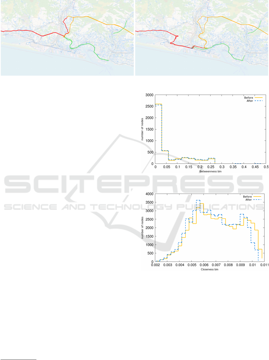
Figure 2: BC: before (left) and after (right) Morandi bridge collapse (detailed vision).

show that the Morandi bridge has one of the highest

in the map, a value of 0.2427, while the maximum

computed value is equal to 0.2556.

Sopra Elevata

, which is an important road that

serves a central area of Genoa Municipality, has a

medium

, a value equal to 0.08. In fact these two

were the most used roads for drivers willing to reach

the centre of the city. Therefore,

results success-

fully capture the fact that many shortest paths were

passing through those nodes. Indeed, the Morandi

bridge was actually one of the most important bridges

(also in graph terms) for the trafﬁc in Liguria.

Figure 1 shows the

of the whole region before

the bridge collapse, with higher values represented

with the red color and lower values represented in blue.

Figure 2 provides a detailed vision of the situation and

the effect of the Morandi bridge collapse is absolutely

relevant. A red important segment disappeared after

the collapse (since the highway was - and still is - inter-

rupted in that point) and alternative city streets (see the

black dots in the map) are now those with the highest

trafﬁc, being the new bridges in the network. As a

consequence, these are also bottlenecks of the entire

network and, indeed, they are the site of trafﬁc jams

during peak trafﬁc hours. More in detail, as we can

see in Figure 2, after the event some central streets of

Genoa became the most important ones. For instance,

Via Cornigliano and Lungomare Canepa moved from

values of 0.0221 and 0.0056 (quite low) to the

new values of 0.4990 and 0.4939, respectively, which

are now the highest values of the entire Liguria road

network.

The two curves in Figure 3 show the

distribu-

tion before and after the collapse of Morandi bridge.

The y-axis represents the number of nodes in a bin (of

size 0.03) with a given value of

; for readability all

nodes with BC equal to 0 are omitted from the plot.

https://it.wikipedia.org/wiki/Strada_sopraelevata_di_

Genova

Figure 3:

distribution: before (solid, yellow) and after

(dashed, blue) Morandi bridge collapse.

Figure 4:

distribution: before (solid, yellow) and after

(dashed, blue) Morandi bridge collapse.

The distribution is right skewed and it can be ob-

served that the tail becomes longer after the collapse,

since new nodes emerge with

values which are out

of the scale before the collapse, as shown by the iso-

lated blue dashed line in the rightmost part of Figure 3.

Changes in the

characteristics of the road net-

work can be observed as well, both at the map level or

by plotting curves. Nodes with high

can be reached

over short distances and Figure 4 shows that, after the

crash, nodes are further away and the overall distances

increased, as daily witnessed by drivers. This is math-

ematically shown in the curves when observing the

Improving the Performance of Road Network Analysis: The Morandi Bridge Case Study

265

shift to left of the blue line w.r.t. the yellow line (e.g.,

nodes show a lower CC and therefore are further away

from each other).

The bin size in Figure 4 is 0.0003 and it can be

observed that, in accord to the theory, the CC results

span over a small range of values, much smaller with

respect to the BC results.

6 CONCLUSIONS AND FUTURE

WORKS

In this work we have presented the computation of

some classical centrality measures for the map of the

region Liguria, before and after the Morandi bridge

collapse, discussing the changes occurred to the street

network. In order to perform an efﬁcient computation

we extended the implementation of the JGraphT library

to support multi-core computation.

The current implementation does not consider any

trafﬁc data but we are planning to extend our work to

build a tool that takes into account also this data source,

possibly by accessing to real trafﬁc data available at

the Municipality level. A second possible extension

will investigate whether a parallel solution could be of

help for the implementation of less classical centrality

measures like those introduced in (Hadas et al., 2017).

In this work we relied on the entire region Liguria

road network model. Thus, the analyses described

in this paper are focussed more on the impact of the

Morandi bridge collapse on “regional travellers” rather

than “city travellers”. As future work we plan to per-

form a multi-scale analysis in order to evaluate the

effects of the crash on different kind of travellers. This

could be very useful to understand the changes for

travellers moving between relevant portions of the city

(e.g., along the Valpolcevera valley

We think that an easy-to-use tool to assess the

inconveniences due to failures in the road network

caused by atmospheric events, temporary accidents,

lasting disasters, or target attacks could be extremely

helpful for local public authorities to simulate the im-

pact of failures before their occurrences.

An analysis of all the side-effects caused by the

collapse of the Morandi bridge is out of the scope of

this paper, but it is worth mentioning that a city like

Genoa, whose economy is heavily based on the ex-

change of goods through its port, in addition to the

paralysis of the private transport system, is nowadays

witnessing an important economic loss which will be

more clear in the next months. Therefore, we think

that a tool that can help to understand the impact of

https://en.wikipedia.org/wiki/Val_Polcevera

random or target failures, and possibly suggest how to

protect the network, for instance by adding some re-

dundancy, should be welcome by the public authorities

and decision makers.

REFERENCES

Castagnari, C., Corradini, F., Angelis, F. D., de Berardinis,

J., Forcina, G., and Polini, A. (2018). Tangramob: an

agent-based simulation framework for validating urban

smart mobility solutions. CoRR, abs/1805.10906.

Glanz, J., Pianigiani, G., White, J., and Patanjali, K. (2018).

Genoa bridge collapse: The road to tragedy. New York

Times. https://www.nytimes.com/interactive/2018/09/

06/world/europe/genoa-italy-bridge.html.

Hadas, Y., Gnecco, G., and Sanguineti, M. (2017). An

approach to transportation network analysis via trans-

ferable utility games. Transportation Research Part B:

Methodological, 105.

Jayaweera, N., Perera, R., and Munasinghe, J. (2017). Cen-

trality measures to identify trafﬁc congestion on road

networks: A case study of Sri Lanka. IOSR Journal of

Mathematics, 13:13–19.

Newman, M. (2018). Networks. OUP Oxford.

Puzis, R., Altshuler, Y., Elovici, Y., Bekhor, S., Shiftan,

Y., and Pentland, A. (2013). Augmented betweenness

centrality for environmentally aware trafﬁc monitor-

ing in transportation networks. Journal of Intelligent

Transportation Systems, 17:91–105.

United-Nations (2016). The world’s cities in 2016. https:

//www.un-ilibrary.org/population-and-demography/

the-world-s-cities-in-2016_8519891f-en.

United-Nations (2018). 68% of the world population

projected to live in urban areas by 2050. https:

//www.un.org/development/desa/en/news/population/

2018-revision-of-world-urbanization-prospects.html.

Windmill (2018). Vehicle sensing: Ten technolo-

gies to measure trafﬁc. http://www.windmill.co.uk/

vehicle-sensing.html.

Zilske, M., Neumann, A., and Nagel, K. (2011). Open-

streetmap for trafﬁc simulation. In Proceedings of 1st

European State of the Map Conference, pages 126–134.

GISTAM 2019 - 5th International Conference on Geographical Information Systems Theory, Applications and Management

266