Energy-optimal Speed Trajectories between Stops and Their Parameter

Dependence

Eduardo F. Mello

and Peter H. Bauer

Department of Electrical Engineering, University of Notre Dame, 275 Fitzpatrick Hall, Notre Dame, U.S.A.

Keywords:

Energy, Efﬁciency, Optimal, Speed Proﬁle, Electric Vehicle.

Abstract:

This paper addresses the problem of energy-optimal vehicle-speed trajectories between stops. The ideal

parameter-dependent trajectory is introduced, and it is shown that it reduces transportation energy drasti-

cally relative to “typical trajectories” seen in trafﬁc. The resulting trajectories can easily be implemented in

self-driving cars and have the potential to signiﬁcantly reduce transportation energy in networked vehicles

and cities. The usage of this energy-optimal speed trajectories between stops can save signiﬁcant amounts of

energy, sometimes in excess of 30% when comparing to conventional trafﬁc ﬂow speed proﬁles. This paper

also addresses the impact that vehicle and segment parameters have on the savings. The role of parameters

such as the air drag coefﬁcient, cross-sectional area, vehicle mass, efﬁciency, segment length, average speed,

as well as acceleration capability are investigated. It is shown that optimizing speed trajectories to minimize

transportation energy consistently results in energy savings. However, diminishing returns are observed for

certain scenarios, such as long, low-speed segments.

1 INTRODUCTION

The advent of self-driving cars, intelligent transporta-

tion, and connected vehicles opens new possibilities

for embedding a variety of algorithms into vehicles

that improve and optimize vehicle operations. This

is in contrast to the current situation where drivers

control vehicle routes and speeds, making the realiza-

tion of optimization algorithms difﬁcult due to lim-

ited acceptance and poor execution by the driver. As

shown in (Stern et al., 2018), by adding a sufﬁcient

portion of autonomous vehicles executing these em-

bedded algorithms, vehicles that do not use such algo-

rithms could be encouraged or even forced to follow

the lead of the self-driven car, at least in dense traf-

ﬁc. This paper explores vehicle-embedded algorithms

that minimize energy usage in typical urban driving

situations, i.e. from stop to stop. While the approach

taken can generally be applied to any type of vehicle,

this paper is limited to electric drive systems. The

proposed concept minimizes the energy expended at

the battery, given the distance and the desired average

speed between two stops. Therefore, the algorithm

chooses the speed-versus-time trajectory that satisﬁes

the given constraints and minimizes transportation en-

https://orcid.org/0000-0002-2339-2305

ergy. In order to carry out this type of optimization,

one needs to know basic vehicle parameters such as

rolling resistance, air drag coefﬁcient, frontal cross-

sectional area, vehicle mass, performance limits, and

efﬁciencies along the drivetrain, all parameters that,

for a given vehicle, are well known. The optimization

algorithm then takes these parameters and the con-

straints and generates the energy-optimal speed pro-

ﬁle. It will be shown that compared to “typical” speed

proﬁles, the optimization results in signiﬁcant energy

savings.

Based on extensive on-road and dynamometer

testing, (Hooker, 1988) created guidelines for how a

driver should operate a vehicle between consecutive

stops; however, in some cases, these guidelines dif-

fered signiﬁcantly, even for similar vehicles. Energy-

optimal speed trajectories were also considered for

large vehicles. However, the analysis was based on

vehicles equipped with internal combustion engines

(ICEs) where there is no regenerative braking and the

efﬁciency of the vehicles was not taken into account

(Henriksson et al., 2017).

In (Mandava et al., 2009), the authors propose an

algorithm that, by using trafﬁc light controller infor-

mation provided to the vehicle by the roadside, speed

recommendations are presented to the driver. The

suggested speeds are generated so that the probabil-

Mello, E. and Bauer, P.

Energy-optimal Speed Trajectories between Stops and Their Parameter Dependence.

DOI: 10.5220/0007747605130520

In Proceedings of the 5th International Conference on Vehicle Technology and Intelligent Transport Systems (VEHITS 2019), pages 513-520

ISBN: 978-989-758-374-2

513

ity of green lights when approaching signalized inter-

sections in arterial roads is maximized, resulting in

energy savings and reduction of emissions due to the

reduction of speed variations and idling times. Ad-

dressing a similar problem, (Schuricht et al., 2011)

developed an algorithm capable of suggesting the

ideal speed proﬁle the driver should adopt in order

to cross a trafﬁc light without having to stop to mini-

mize the energy consumption. This research differs

from (Mandava et al., 2009) by using information

from trafﬁc light controllers and data from a queue

length estimator. A slightly different solution was

proposed by (Nunzio et al., 2013). Instead of sim-

ply avoiding stops in a trafﬁc corridor, the developed

algorithm evaluates multiple available no-stop speed

proﬁles and then chooses the most efﬁcient scenario.

With a focus on plug-in hybrid electric vehicles,

(Qi et al., 2017) created a system capable of opti-

mizing the speed proﬁle in a signalized arterial road

and co-optimizing the vehicle dynamics and hybrid

powertrain operations. In a similar approach, the au-

thors in (Barth et al., 2011) calculate the speed pro-

ﬁle which minimizes fuel consumption in a signal-

ized arterial road for a vehicle equipped with an inter-

nal combustion engine by reducing the total tractive

power demand and the idling time.

A separate line of research related to the work pro-

posed in this paper is presented by (Yi and Bauer,

2017b), where the impact of environmental factors

such as wind speed, rolling resistance, and temper-

ature on an electric vehicle’s energy consumption is

analyzed. In (Yi and Bauer, 2018), the authors pro-

pose a robust optimization model that exploits these

environmental factors to generate an optimal speed

proﬁle. Finally, the result in (Yi and Bauer, 2017a)

estimates the energy consumption of an electric vehi-

cle based on three parameters (powertrain efﬁciency,

wind speed, and rolling resistance), with variable de-

gree of accuracy depending on energy reserves.

2 THE MODEL

In order to describe the expended energy of a vehi-

cle’s speed trajectory, one needs to consider all power-

absorbing components, i.e. air drag, rolling resis-

tance, acceleration/deceleration of the vehicle and hill

climbing. Therefore, based on the models presented

in (Yi and Bauer, 2017b), the power at the wheel,

denoted as P

wheel

can be written as shown in (1)

where m, v(t), ˙v(t), C

, and A are the vehicle’s mass

(which also models and includes the driveline iner-

tia), speed, acceleration, frontal drag coefﬁcient, and

cross-sectional area, respectively. ρ is the air density,

is the coefﬁcient of rolling resistance, and g is the

gravitational acceleration. In this analysis we assume

a ﬂat surface, i.e. no hill climbing.

wheel

(t) = mv(t) ˙v(t) +

Aρv(t)

+ mg f

v(t) (1)

The power balance equation for forward motion

(2) and for regenerative breaking (3), i.e. reverse

power ﬂow, are given by:

bat

(t) =

f rw

wheel

(t)) for P

wheel

> 0 (2)

bat

(t) = η

reg

wheel

(t)) for P

wheel

< 0 (3)

where P

bat

(t) is the power at the battery, η

f rw

is the

vehicle’s efﬁciency for forward power ﬂow, and η

reg

is the vehicle’s efﬁciency in reverse power ﬂow. The

battery energy, E

bat

, for the power ﬂow is therefore

given by (4).

bat

(t)dt (4)

Discretizing the energy equation in (4), a constant

approximation can be used for all power absorbing

components. The acceleration term is approximated

by the difference in kinetic energy values at each dis-

tance segment. Each discretized energy segment, ∆E,

is described by (5), where v

denotes a constant-speed

segment and ∆t a sampling time.

∆E



n+1

−v



Aρv

∆t + mg f

∆t (5)

The optimization problem can then be formulated

in a piecewise discretized form, as shown in (6) and

(7). N represents the total number of segments and

∆E

denotes an energy segment where the forward

and reverse power ﬂow efﬁciencies are accounted for.

∆E

(

f rw

∆E

f or ∆E > 0

reg

∆E

f or ∆E ≤ 0

(6)

E =

∑

n=1

∆E

(7)

Finally, the optimization problem can then be

written as shown in (8).

min

s.t.

∑

n=1

= v

avg

0 ≤ v

≤ v

max

≤

n+1

− v

∆t

≤ a

max

∀ n ∈ {1, ...,N − 1}

max

≤

−v

∆t

≤ a

max

i f n = N

(8)

VEHITS 2019 - 5th International Conference on Vehicle Technology and Intelligent Transport Systems

514

where v

avg

is the desired average speed, v

max

is the

maximum allowed speed, d

max

is the maximum allow-

able deceleration, and a

max

is the maximum allowable

acceleration.

3 SIMULATION RESULTS AND

OPTIMIZATION

The optimization problem expressed in (8) was imple-

mented using the fmincon solver from MATLAB with

the Sequential Quadratic Programming (SQP) algo-

rithm. In order to verify if the optimization proposed

in this paper would be applicable to various vehicles

and scenarios, a number of simulations with different

parameter sets were performed. Initially, a short seg-

ment was tested with two vehicle models, one based

on a Nissan Leaf and the second based on a Tesla

Model S. Then, parameters such as average speed of

the vehicle, segment length, maximum tolerable acce-

lartions and decelerations, and the vehicle efﬁciency

were varied. Finally a larger sample of vehicles in a

number of different scenarios were tested.

3.1 Approximation of a Real Scenario

In order to deﬁne a baseline for typical trafﬁc ﬂow, the

Federal Test Procedure (FTP-75) drive cycle was an-

alyzed. To generate the typical trafﬁc proﬁle the drive

cycle was divided into segments (corresponding to the

periods for which the car is movement), normalized in

time and speed, and then all segments were averaged.

The curve generated was then approximated by

an exponential acceleration until it reached the max-

imum speed followed by a parabolic deceleration.

Both curves are shown in Figure 1 where the curve

“Real scenario” is extracted from the FTP-75 drive

cycle and the curve “Typical trafﬁc” shows the ap-

proximated curve.

Figure 1: Speed vs. time of the “Real scenario” extracted

from FTP-75 and approximated “Typical trafﬁc” ﬂow.

3.2 Optimization Results for Urban

Trafﬁc

The proposed optimization was used for a couple of

vehicles in order to verify the robustness of the results

relative to vehicle and infrastructure parameters. The

ﬁrst tested case was for a vehicle with a parameter set

based on a Nissan Leaf in a 300-meter segment. The

second vehicle model utilized was based on a Tesla

Model S in a segment with the same 300-meter in

length.

3.2.1 Nissan Leaf

The baseline case is investigated for a midsize electric

vehicle (EV), which has its parameter set based on the

Nissan Leaf. The vehicle data set is given as follows:

m = 1525kg, f

= 0.01, C

= 0.29, and A = 2.27m

The average forward and reverse power ﬂow efﬁcien-

cies were approximated as η

f rd

= 0.7, and η

reg

= 0.2.

The speed trajectories for the approximation of the

typical trafﬁc ﬂow and the optimized trajectory are

shown in Figure 2. Figure 3 shows the acceleration

proﬁle necessary to realize the aforementioned speed

proﬁles. And ﬁnally, the energy utilized by the vehi-

cle in each case is shown Figure 4.

In this simulation, the constraints imposed on the

optimizer were: the length between two consecu-

tive stops was chosen to be 300m, the average speed

throughout the proﬁle had to be equal to 10m/s, the

maximum acceleration 4.6m/s

, the maximum decel-

eration -2m/s

, and ﬁnally, the initial and ﬁnal speeds

equal to zero.

The results obtained show that the optimized

speed proﬁle consumes 179.9kWs while the typical

trafﬁc baseline uses 235.4kW s, a 23.59% reduction.

This demonstrates that the optimization proposed in

this paper has the potential of drastically minimiz-

ing the energy consumption in a route with necessary

stops.

3.2.2 Tesla Model S

The optimization was then repeated for a vehicle with

a parameter set based on the Tesla Model S. This vehi-

cle was chosen as it is another typical electric vehicle

and it has higher maximum acceleration and decelera-

tion than a Nissan Leaf. The parameter values utilized

are: m = 2018kg, f

= 0.01, C

= 0.24, and A = 2.8m

The average forward and reverse power ﬂow efﬁcien-

cies were approximated as η

f rd

= 0.7, and η

reg

= 0.2.

The distance between the two stops was kept at 300m.

The acceleration of the vehicle was limited to 8m/s

and the deceleration to -2.5m/s

Energy-optimal Speed Trajectories between Stops and Their Parameter Dependence

515

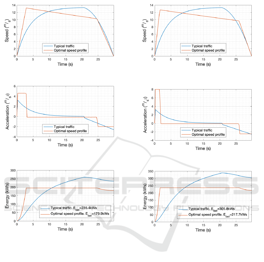
Figure 2: Speed for the “Typical trafﬁc” and “Optimal

speed” proﬁles for a Nissan Leaf.

Figure 3: Acceleration for the “Typical trafﬁc” and “Opti-

mal speed” proﬁles for a Nissan Leaf.

Figure 4: Energy for the “Typical trafﬁc” and “Optimal

speed” proﬁles for a Nissan Leaf.

As already seen in Figure 2, the optimal speed

proﬁle for this vehicle, Figure 5, is characterized by

three different stages (acceleration, coasting, and de-

celeration) until a complete stop is reached. With the

aforementioned parameters, the optimizer produced a

speed proﬁle which uses 217.7kWs, as seen in Fig-

ure 7. This value is 28.81% less than the one obtained

for the typical trafﬁc baseline, which used 305.8kWs,

saving 88.1kW s.

As expected, since the Tesla Model S is a heav-

ier vehicle with a larger cross-sectional area, it uses

more energy than the Nissan Leaf in each of the driv-

ing schedules, i.e. typical trafﬁc baseline and optimal

speed proﬁle. However, the Tesla Model S was able

to achieve greater percentage savings when compared

to the Nissan Leaf due to its greater acceleration and

deceleration.

Figure 5: Speed for the “Typical trafﬁc” and “Optimal

speed” proﬁles for a Tesla Model S.

Figure 6: Acceleration for the “Typical trafﬁc” and “Opti-

mal speed” proﬁles for a Tesla Model S.

Figure 7: Energy for the “Typical trafﬁc” and “Optimal

speed” proﬁles for a Tesla Model S.

3.3 The Effects of Segment Length and

Average Speed

Two simulations were performed in order to verify

the effects of average speed and segment length in the

optimized speed proﬁles. Both simulations were per-

formed for the same vehicle with parameters based on

a Tesla Model S.

3.3.1 Midrange Segment Length and High

Speed

The initial scenario simulated was a segment of

1000m at an average speed of 20m/s. The stop-to-

stop length and average speed were chosen in order to

keep the accelerations and decelerations in our base-

lines within realistic margins. One important aspect

VEHITS 2019 - 5th International Conference on Vehicle Technology and Intelligent Transport Systems

516

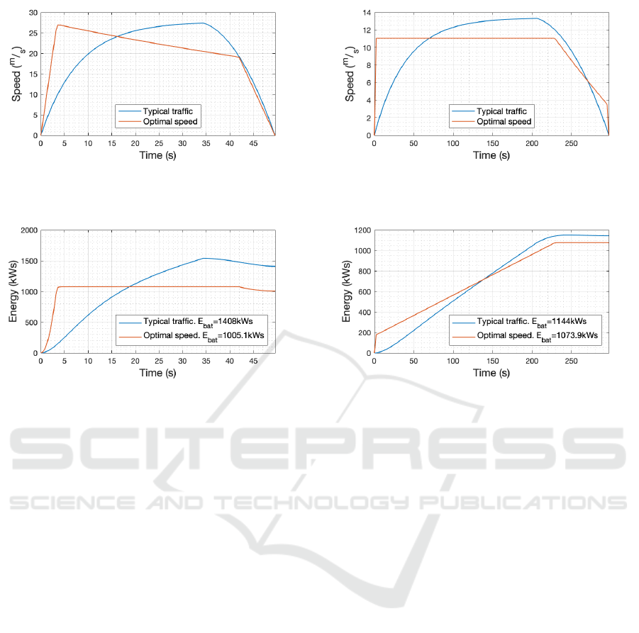
Figure 8: Speed for “Typical trafﬁc” and “Optimal speed”

proﬁles for a stop-to-stop segment length of 1000m and av-

erage speed of 20m/s.

Figure 9: Energy for “Typical trafﬁc” and “Optimal speed”

proﬁles for a stop-to-stop segment length of 1000m and av-

erage speed of 20m/s.

to be kept in mind is that the speed proﬁle baselines

must have realizable accelerations in order to be com-

pared to the results of the optimizer, which has re-

alizable accelerations as constraints. In this case, as

shown in Figures 8 and 9, it was observed that the op-

timized speed proﬁle saves 402.9kW s when compared

to the typical trafﬁc baseline, which is equivalent to

28.61%. The total energy used in the simulation was

1408kW s for the baseline and 1005.1kW s for the op-

timal speed proﬁle. Based on these results, it is clear

that the optimizer is capable of generating signiﬁcant

savings even for higher speed scenarios.

3.3.2 Long Segment Length and Low Speed

Figures 10 and 11 show the simulation for a segment

length of 3000m at a speed of 10m/s, i.e. half of the

speed used in the previous case. The results obtained

from the optimizer show savings of 6.13% when com-

pared to the typical trafﬁc baseline. This value corre-

sponds to 70.14kWs. With the information provided

by this simulation, it can be concluded that this op-

timization has diminished results when the length of

the stop-to-stop segment is drastically increased.

Figure 10: Speed for “Typical trafﬁc” and “Optimal speed”

proﬁles for a stop-to-stop segment length of 3000m and av-

erage speed of 10m/s.

Figure 11: Energy for “Typical trafﬁc” and “Optimal speed”

proﬁles for a stop-to-stop segment length of 3000m and av-

erage speed of 10m/s.

3.4 The Effects of Maximum Tolerable

Acceleration and Deceleration

As seen in Figure 8 and Figure 10, the optimal speed

proﬁle is typically characterized by three to four

pronounced segments: acceleration, constant speed

(which in certain circumstances may not exist), coast-

ing, and deceleration. These well-deﬁned segments

raise the question of what the effects of the acceler-

ation and deceleration limits (constraints of the opti-

mizer) are.

To verify the effects of the aforementioned lim-

its, the simulation in section 3.2.2 was repeated with

new limits for the acceleration and deceleration con-

straints. The segment length was kept at 300m with

an average speed of 10m/s. The acceleration of the

vehicle was limited to 4m/s

and the deceleration to

-1.25m/s

. These values correspond to half of the

ones used in section 3.2.2. With these parameters,

the optimizer produced a speed proﬁle which uses

274.4kW s. This value is 10.44% smaller than the

one obtained for the typical trafﬁc baseline, saving

31.98kW s. The optimal speed proﬁle generated can

be seen in Figures 12 and 13.

In this simulation, the acceleration and decelera-

tion limits were set to half of the values utilized in sec-

tion 3.2.2. This change caused an increase in energy

Energy-optimal Speed Trajectories between Stops and Their Parameter Dependence

517

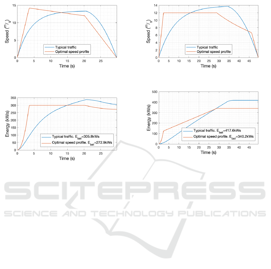
Figure 12: Speed for the “Typical trafﬁc” and “Optimal

speed” proﬁles for a Tesla Model S with reduced maximum

acceleration and deceleration in a 300-meter segment.

Figure 13: Energy for the “Typical trafﬁc” and “Optimal

speed” proﬁles for a Tesla Model S with reduced maximum

acceleration and deceleration in a 300-meter segment.

consumption of 55.2kW s. This energy increase corre-

sponds to 18.37% of the energy utilized by the vehi-

cle when higher acceleration and deceleration were

allowed. Thus, it can be stated that by increasing

the maximum tolerable acceleration and deceleration,

higher savings can be achieved.

3.5 The Effects of Vehicle Efﬁciency

3.5.1 Highly Inefﬁcient Vehicle

In order to validate the robustness of the results with

respect to the vehicle model, another set of simula-

tions was run. The ﬁrst simulation represents a highly

inefﬁcient vehicle with the following parameters: m =

1000kg, f

= 0.015, C

= 1, and A = 3m

, η

f rd

= 0.6,

and η

reg

= 0. The acceleration was limited to 5m/s

and the deceleration to -2m/s

. The segment length

was set to 500m with an average speed of 10m/s.

The simulation output showed a signiﬁcant im-

provement over the speed proﬁle baselines for the in-

efﬁcient vehicle, as seen in Figures 14 and 15. The

optimized speed proﬁle was able to save 77.4kW s

over the typical trafﬁc ﬂow baseline, which corre-

sponds to 18.52% of improvement. Therefore, the

algorithm showed to be a very plausible option for

reducing the energy consumption of highly inefﬁcient

electric vehicles.

Figure 14: Speed for the “Typical trafﬁc” and “Optimal

speed” proﬁles for a highly inefﬁcient vehicle.

Figure 15: Energy for the “Typical trafﬁc” and “Optimal

speed” proﬁles for a highly inefﬁcient vehicle.

3.5.2 Highly Efﬁcient Vehicle

The second simulation assumes a model of a highly

efﬁcient vehicle. Its parameters were deﬁned as: m

= 2000kg, f

= 0.008, C

= 0.25, A = 2m

, η

f rd

0.9, and η

reg

= 0.5. The acceleration was once again

limited to 5m/s

and the deceleration to -2m/s

. The

segment length and average speed were also kept the

same—500m and 10m/s.

With the parameters described above, drops in en-

ergy consumption of 26.73% with respect to the typi-

cal trafﬁc baseline were observed (Figures 16 and 17).

These savings correspond to 56.29kW s. Thus, it can

be assumed that the optimization is capable of signif-

icant energy savings for efﬁcient and inefﬁcient elec-

tric vehicles, where greater savings are observed for

an efﬁcient vehicle.

3.6 Additional Vehicle Models and the

Impact of the Segment Length

A ﬁnal set of simulations was performed in order

to compare a number of different scenarios where

the vehicle parameters, segment length, and average

speed were varied. Five vehicle parameter sets were

utilized and they are speciﬁed in Table 1. Vehicle type

1 has a parameter set similar to the parameters of a

Tesla Model S and vehicle type 2 has similar param-

eters to a Nissan Leaf. Parameters such as vehicle

VEHITS 2019 - 5th International Conference on Vehicle Technology and Intelligent Transport Systems

518

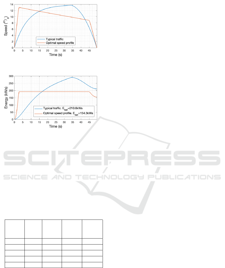
Figure 16: Speed for the “Typical trafﬁc” and “Optimal

speed” proﬁles for a highly efﬁcient vehicle.

Figure 17: Energy for the “Typical trafﬁc” and “Optimal

speed” proﬁles for a highly efﬁcient vehicle.

mass, cross-sectional area multiplied by air drag co-

efﬁcient, efﬁciencies, and maximum acceleration and

deceleration were modiﬁed in order to analyze the

impact they have on transportation energy savings.

Vehicle type 3 is a variation of vehicle type 2 with

high maximum acceleration and deceleration. Vehi-

cle types 4 and 5 have extreme parameter sets with

high mass and low Cd

for the former and low mass

and high Cd

for the latter to illustrate the effects of

these vehicle parameters.

Table 1: Vehicle parameters utilized in simulations.

Vehicle

Mass

(kg)

)

Max.

acceler.

(m/s

)

Max.

deceler.

(m/s

)

Type 1 2,018 0.6720 8 2.5

Type 2 1,525 0.6583 4.6 2

Type 3 1,525 0.6583 8 2.5

Type 4 2,500 0.5 4.6 2

Type 5 800 2.0 4.6 2

A segment length of 300 meters was used in most

simulations since it is a typical length for a suburban

block (Hooker, 1988).

Table 2 shows the results obtained. In all cases,

the optimal trajectory results in energy savings. These

savings demonstrate the robustness of the optimiza-

tion results with respect to the vehicle parameter set.

However, the segment length has a signiﬁcant impact

on energy savings. Improvements ranging from 6%

to 41% were observed in this set of simulations.

These results show that energy savings are partic-

ularly high for short distance segments. Also, vehi-

cles capable of accelerating rapidly have greater sav-

ings in transportation energy, which is especially pro-

nounced in short segments. This can be seen by notic-

ing that Vehicle type 3 obtains higher savings than Ve-

hicle type 2 (mostly identical vehicles with exception

of the acceleration capabilities). Also, Vehicle type 1

obtained higher savings than Vehicle type 2 in almost

all scenarios. Finally, it can be observed that high sav-

ings are also obtained for vehicles traveling at higher

average speeds in long segments.

4 CONCLUSIONS

This paper shows that optimized speed trajectories

between stops can lead to signiﬁcant transportation-

energy savings. Depending on the distance, average

speed, and vehicle parameters, energy savings can

reach approximately 40% relative to typically seen

speed proﬁles. It is important to note that savings are

dependent on the speed proﬁle used as the baseline.

It was further shown that the optimal speed proﬁle

usually has three to four distinct segments: acceler-

ation, constant speed (which is not present for short

distances), coasting, and deceleration. All speed tra-

jectories show the same trend regardless of the param-

eter set: the more energy that can be expended at the

beginning of the stop-to-stop segment, the higher the

savings.

In addition, this paper examined the effects of dif-

ferent vehicle parameters and operating conditions on

transportation energy savings relative to conventional

stop-to-stop speed trajectories. In all cases, the op-

timal trajectory results in energy savings, which in

the simulations presented in this paper range from 6%

to 41%, depending on the constraints and parameters

chosen. This is only possible due to the robust na-

ture of the optimization results obtained with respect

to vehicle and infrastructure parameters. Energy sav-

ings are particularly high for short distance segments.

Also, vehicles capable of accelerating rapidly have

greater savings in transportation energy, which is es-

pecially pronounced in short segments.

Therefore, the impact on self-driving electric ve-

hicles (EVs) and the associated transportation infras-

tructure is twofold: range improvement of EVs due to

lower energy expenditure in urban driving situations,

and less power demand from the grid to charge EVs.

It is important to note that the speed controller that

executes the optimal trajectory needs to communicate

Energy-optimal Speed Trajectories between Stops and Their Parameter Dependence

519

Table 2: Energy consumption for different vehicles and segment lengths.

Energy utilized

Vehicle

Forward

Power

Flow

Efﬁciency

Reverse

Power

Flow

Efﬁciency

Average

speed

(m/s)

Segment

length

(m)

Typical trajectory

(kW s)

Optimal trajectory

(kW s)

Energy

saved

Vehicle type 1 0.7 0.2

300 305.8 217.7 28.81 %

500 375.4 253.7 32.42 %

1,000 519.7 393.7 24.24 %

3,000 1,144.0 1,073.9 6.13 %

18 3,000 2,043.7 1,643.8 19.57 %

Vehicle type 2 0.7 0.2

300 235.4 179.9 23.59 %

500 290.9 203.9 29.91 %

1,000 407.7 314.4 22.88 %

3,000 915.1 853.8 6.7 %

18 3,000 1,695.7 1,392.7 17.87 %

Vehicle type 3

.7 .2 10 300

235.4 167.9 28.67 %

Vehicle type 4 449.2 291.9 35.02 %

Vehicle type 5 234.0 137.6 41.20 %

with the self-driving software in order to prevent ac-

cidents. Even though the proposed speed trajectories

have strong accelerations, the speeds in urban scenar-

ios are generally around 50km/h or less.

REFERENCES

Barth, M., Mandava, S., Boriboonsomsin, K., and Xia, H.

(2011). Dynamic eco-driving for arterial corridors.

In 2011 IEEE Forum on Integrated and Sustainable

Transportation Systems, pages 182–188.

Henriksson, M., Fl

ardh, O., and M

artensson, J. (2017). Op-

timal speed trajectories under variations in the driving

corridor. IFAC-PapersOnLine, 50(1):12551 – 12556.

20th IFAC World Congress.

Hooker, J. (1988). Optimal driving for single-vehicle fuel

economy. Transportation Research Part A: General,

22(3):183 – 201.

Mandava, S., Boriboonsomsin, K., and Barth, M. (2009).

Arterial velocity planning based on trafﬁc signal in-

formation under light trafﬁc conditions. In 2009 12th

International IEEE Conference on Intelligent Trans-

portation Systems, pages 1–6.

Nunzio, G. D., de Wit, C. C., Moulin, P., and Domenico,

D. D. (2013). Eco-driving in urban trafﬁc networks

using trafﬁc signal information. In 52nd IEEE Con-

ference on Decision and Control, pages 892–898.

Qi, X., Wu, G., Hao, P., Boriboonsomsin, K., and Barth,

M. J. (2017). Integrated-connected eco-driving sys-

tem for phevs with co-optimization of vehicle dynam-

ics and powertrain operations. IEEE Transactions on

Intelligent Vehicles, 2(1):2–13.

Schuricht, P., Michler, O., and B

aker, B. (2011). Efﬁciency-

increasing driver assistance at signalized intersections

using predictive trafﬁc state estimation. In 2011 14th

International IEEE Conference on Intelligent Trans-

portation Systems (ITSC), pages 347–352.

Stern, R. E., Cui, S., Monache, M. L. D., Bhadani, R.,

Bunting, M., Churchill, M., Hamilton, N., Haulcy,

R., Pohlmann, H., Wu, F., Piccoli, B., Seibold, B.,

Sprinkle, J., and Work, D. B. (2018). Dissipation

of stop-and-go waves via control of autonomous ve-

hicles: Field experiments. Transportation Research

Part C: Emerging Technologies, 89:205 – 221.

Yi, Z. and Bauer, P. H. (2017a). Adaptive multiresolu-

tion energy consumption prediction for electric ve-

hicles. IEEE Transactions on Vehicular Technology,

66(11):10515–10525.

Yi, Z. and Bauer, P. H. (2017b). Effects of environmen-

tal factors on electric vehicle energy consumption: a

sensitivity analysis. IET Electrical Systems in Trans-

portation, 7(1):3–13.

Yi, Z. and Bauer, P. H. (2018). Energy aware driving: Op-

timal electric vehicle speed proﬁles for sustainability

in transportation. IEEE Transactions on Intelligent

Transportation Systems, pages 1–12.

VEHITS 2019 - 5th International Conference on Vehicle Technology and Intelligent Transport Systems

520